Structural analysis
This is a detailed tutorial for structural analysis of individual images and movies using the the SarcAsM Python package.
Detailed documentation of all functions with parameters and output see API reference.
A detailed list of all analyzed features can be found here.
Download the Jupyter notebook here.
[1]:
from sarcasm import *
from matplotlib import pyplot as plt
Initialization of SarcAsM object
If SarcAsM is not able to automatically read the pixel size from the tif-file, an error is raised and the pixel size in µm must be entered manually by Structure(filepath, pixelsize=0.1). Additional metadata can be added upon initialization by keyword arguments, e.g., Structure(filepath, cell_line='WT').
All parameters see API reference.
[2]:
# enter path of tif-file, can be both single image and movie
filepath = '../../_test_data/20211115_ACTN2_CMs_96well_control_12days.tif'

# initialize Structure object
sarc = Structure(filepath)
Prediction of sarcomere Z-bands and cell area by deep learning
SarcAsM predicts Z-bands, M-bands, sarcomere orientation and cell mask from fluorescent images using a U-Net convolutional neural network, by sarc.detect_sarcomeres(). By default, a generalist model trained on a diverse data set, is used. To specify the model, adapt model_path.
All parameters see API reference.
[3]:
# detect sarcomeres and cell mask
sarc.detect_sarcomeres(max_patch_size=(2048, 2048))
Predicting sarcomeres ...
100%|██████████| 50/50 [01:52<00:00, 2.25s/it]
[4]:
# visualize sarcomere z-bands and cell mask
fig, axs = plt.subplots(ncols=3, figsize=(12, 4), dpi=300)

frame = 33

# image
Plots.plot_image(axs[0], sarc, frame=frame, title='Image')

# z-bands
Plots.plot_z_bands(axs[1], sarc, frame=frame, title='Z-bands', cmap='Grays_r')

# cell mask
Plots.plot_cell_mask(axs[2], sarc, frame=frame, title='Cell mask')

plt.show()
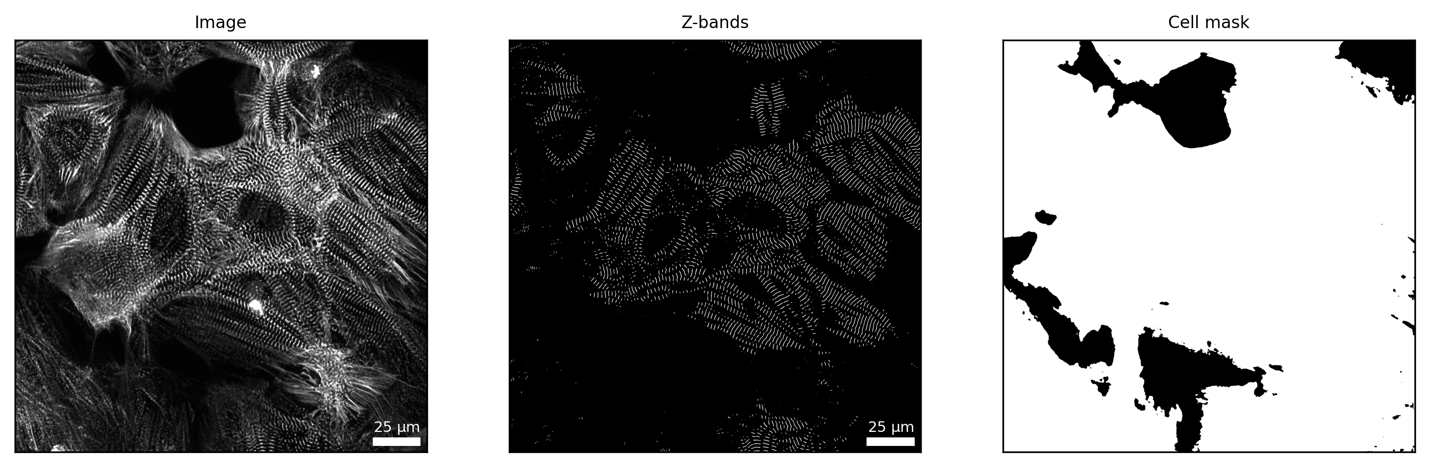
Analysis of cell mask
By sarc.analyze_cell_mask(), SarcAsM analyzes the cell mask area, the area ratio occupied by cells and the mean cell intensity in each image.
Function parameters are described in API reference.
[5]:
# analyze cell mask
sarc.analyze_cell_mask()
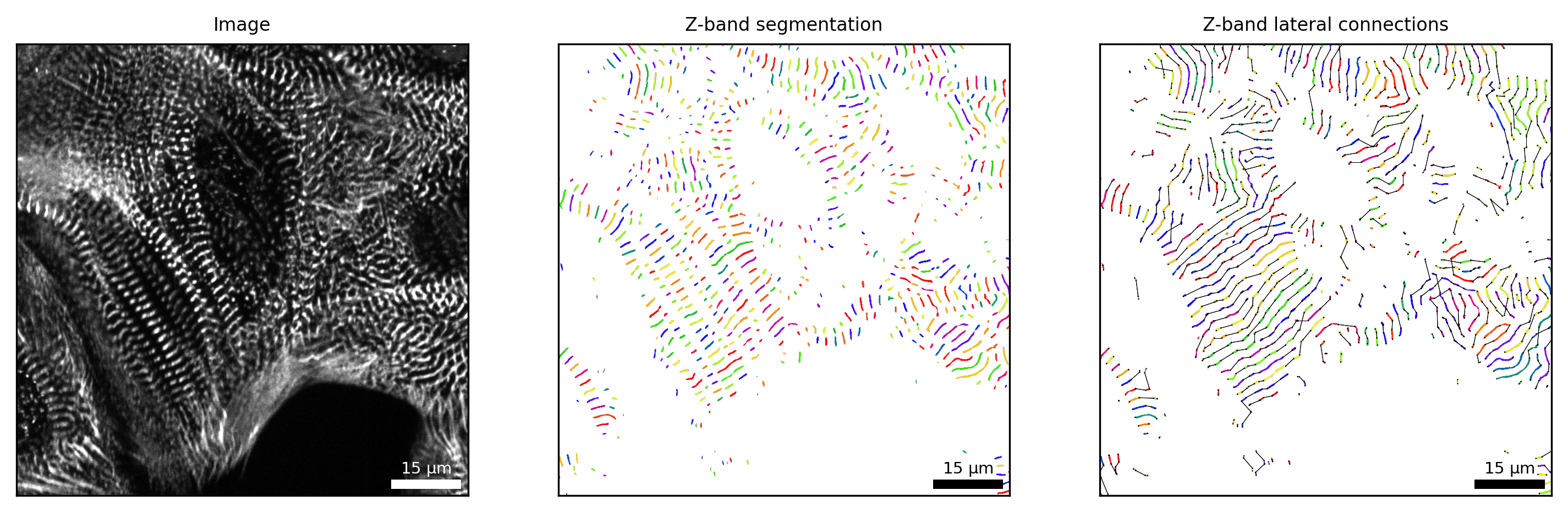
Analysis of sarcomere Z-bands
By sarc.analyze_z_bands(), SarcAsM segments individual Z-bands and analyzes their length, intensity, orientation and straightness as well as the lateral alignment and distance between neighboring Z-bands and properties of laterally aligned Z-bands.
Function parameters are described in API reference.
[6]:
# analyze z-bands
sarc.analyze_z_bands()
Starting Z-band analysis...
100%|██████████| 50/50 [02:07<00:00, 2.54s/it]
[7]:
# visualize z-band segmentation and lateral connections
fig, axs = plt.subplots(ncols=3, figsize=(12, 4), dpi=300)

frame = 33

xlim, ylim = (300, 1200), (300, 1200)

# image
Plots.plot_image(axs[0], sarc, frame=frame, title='Image')
axs[0].set_xlim(xlim)
axs[0].set_ylim(ylim)

# z-band segmentation
Plots.plot_z_segmentation(axs[1], sarc, frame=frame, title='Z-band segmentation')
axs[1].set_xlim(xlim)
axs[1].set_ylim(ylim)

# lateral connections
Plots.plot_z_lateral_connections(axs[2], sarc, frame=frame, title='Z-band lateral connections')
axs[2].set_xlim(xlim)
axs[2].set_ylim(ylim)

plt.show()
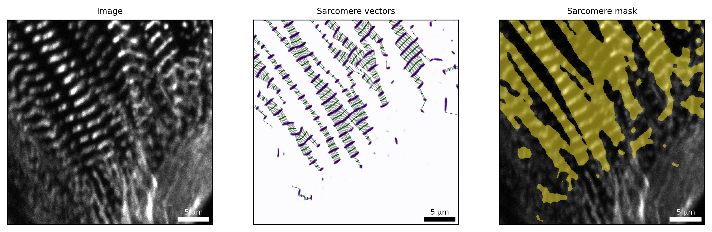
Analysis of sarcomere vectors
By sarc.analyze_sarcomere_vectors(), SarcAsM locally analyzes sarcomere lengths and orientations, based on sarcomere Z-bands and orientations detected by deep learning.
All parameters are described in API reference.
[8]:
# analysis of sarcomere vectors
sarc.analyze_sarcomere_vectors()
Starting sarcomere length and orientation analysis...
100%|██████████| 50/50 [02:17<00:00, 2.75s/it]
[9]:
# visualize sarcomere vectors
fig, axs = plt.subplots(ncols=3, figsize=(12, 4), dpi=300)

frame = 33

xlim, ylim = (500, 800), (400, 700)

# image
Plots.plot_image(axs[0], sarc, frame=frame, title='Image')
axs[0].set_xlim(xlim)
axs[0].set_ylim(ylim)

# sarcomere vectors (adjust parameters 'linewidths' and 's_points')
Plots.plot_sarcomere_vectors(axs[1], sarc, frame=frame, s_points=10, title='Sarcomere vectors')
axs[1].set_xlim(xlim)
axs[1].set_ylim(ylim)

# sarcomere mask
Plots.plot_sarcomere_mask(axs[2], sarc, frame=frame, title='Sarcomere mask')
axs[2].set_xlim(xlim)
axs[2].set_ylim(ylim)

plt.show()
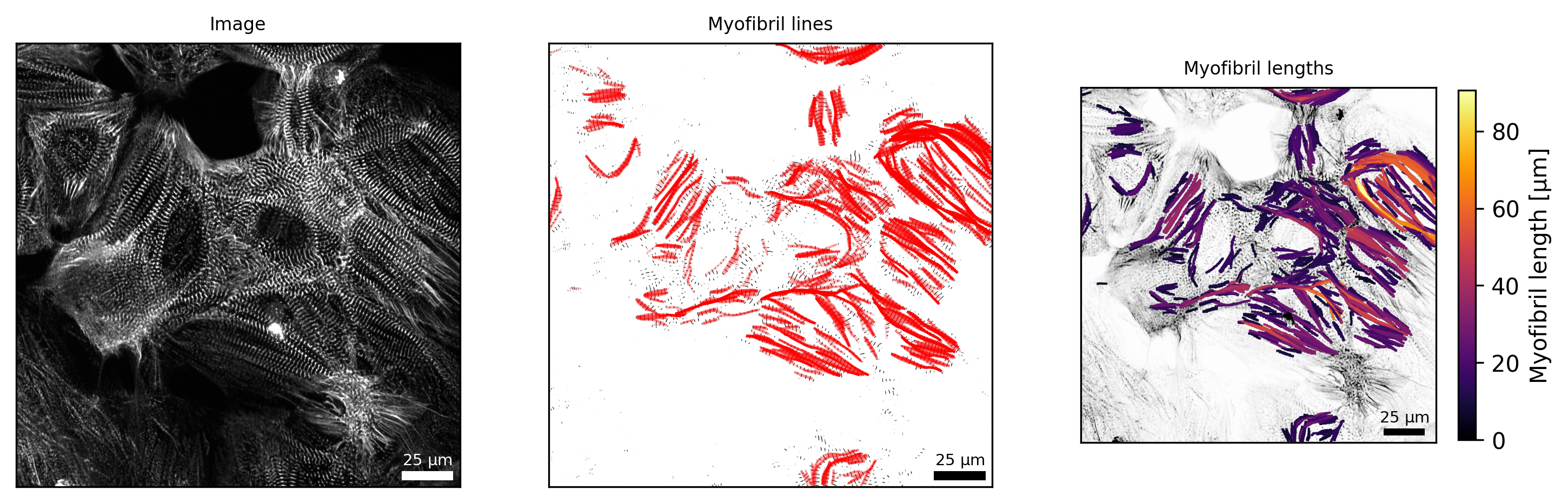
Analysis of myofibrils
By sarc.analyze_myofibrils(), SarcAsM estimates the position, length and curvature of myofibrils using a custom line growth algorithm based on sarcomere vectors.
All parameters are described in API reference.
[10]:
# myofibril analysis
sarc.analyze_myofibrils()
Starting myofibril line analysis...
100%|██████████| 50/50 [01:29<00:00, 1.80s/it]
[11]:
# visualize myofibrils
fig, axs = plt.subplots(ncols=3, figsize=(12, 4), dpi=300)

frame = 33

# image
Plots.plot_image(axs[0], sarc, frame=frame, title='Image')

# myofibril lines
Plots.plot_myofibril_lines(axs[1], sarc, frame=frame, title='Myofibril lines')

# myofibril length map
Plots.plot_myofibril_length_map(axs[2], sarc, frame=frame, title='Myofibril lengths')

plt.show()
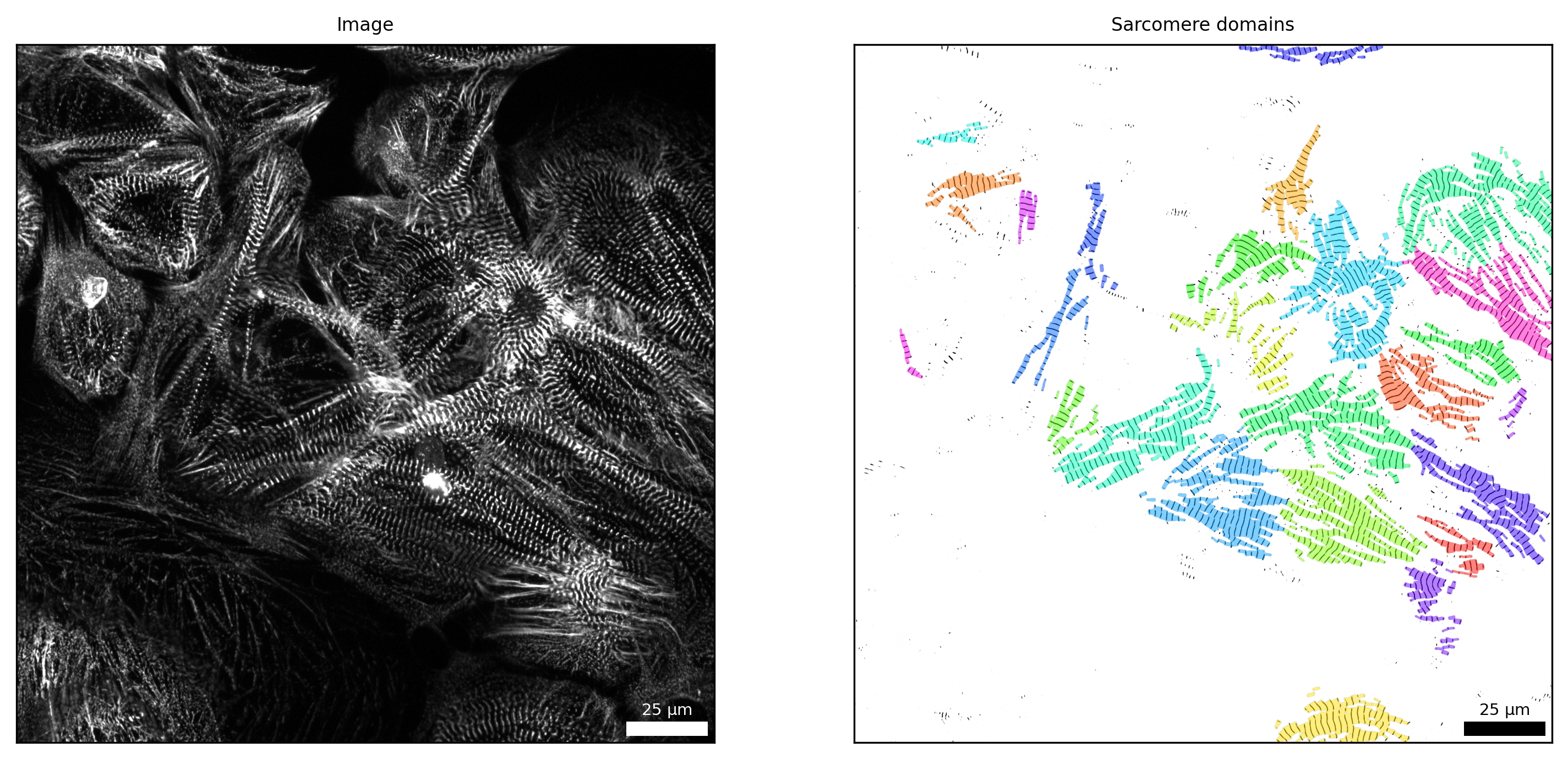
Clustering of sarcomere domains
By sarc.analyze_sarcomere_domains(), SarcAsM groups sarcomere vectors into spatial domains with similar orientation using clustering.
All parameters are described in API reference.
[12]:
# analyze sarcomere domains
sarc.analyze_sarcomere_domains()
Starting sarcomere domain analysis...
100%|██████████| 50/50 [01:01<00:00, 1.24s/it]
[13]:
# visualize sarcomere domains
fig, axs = plt.subplots(ncols=2, figsize=(12, 6), dpi=300)

frame = 30

# image
Plots.plot_image(axs[0], sarc, frame=frame, title='Image')

# myofibril lines
Plots.plot_sarcomere_domains(axs[1], sarc, frame=frame, title='Sarcomere domains')

plt.show()