Télécom Paris

From Reconstruction to Reasoning

Télécom Paris

From Reconstruction
to ReasoningStructured 3D Representations

Bingchen Gong

LIX, École Polytechnique

21 September 2026

Foundations for the research programme From Video to Animatable and Efficient 3D Worlds

Bingchen Gong · LIX, École Polytechnique · 21 September 20261
Motivation

Editing captured scenes
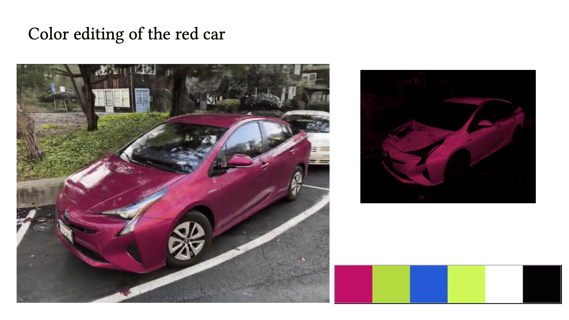
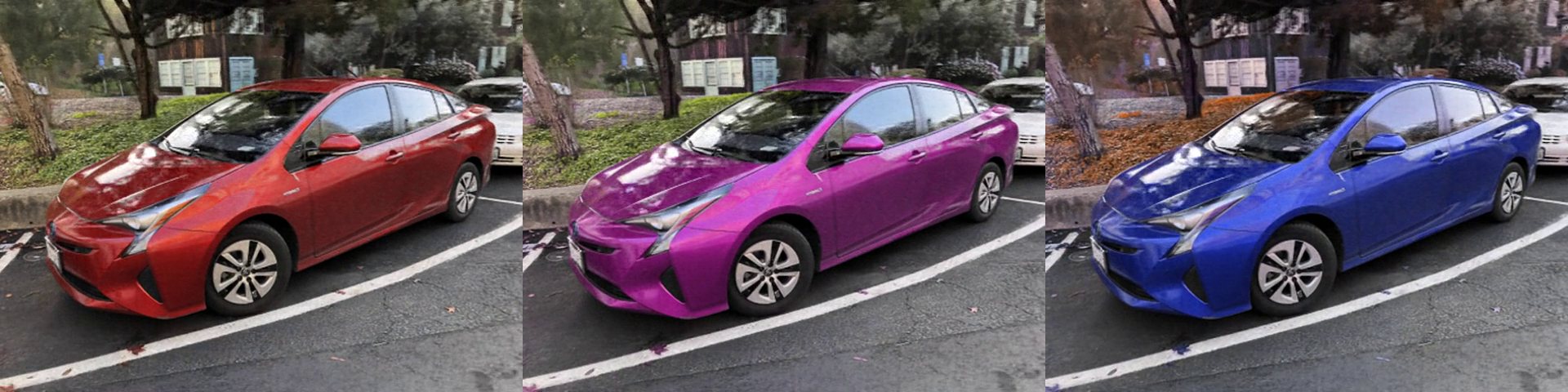
RecolorNeRF demonstration: editing a palette entry recolors the car; the active layer is shown at the right and the palette below
RecolorNeRF: edit colors through a palette
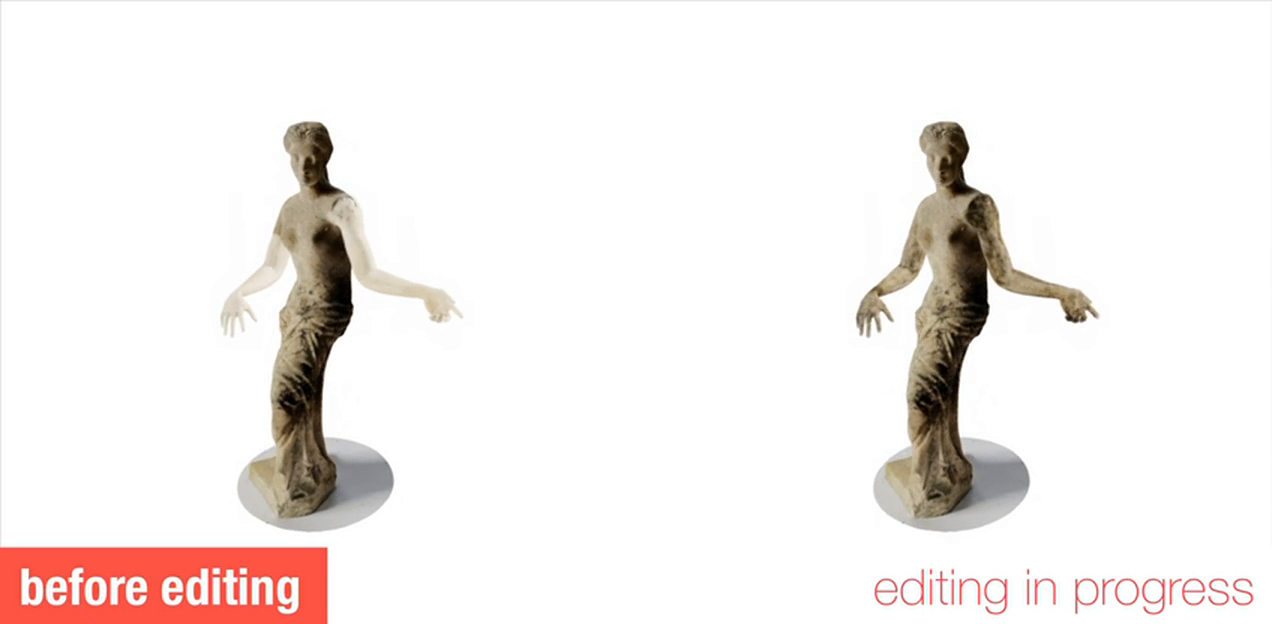
SeamlessNeRF demonstration: arms from another radiance field attached to a statue, before editing and with appearance propagated across the seam
SeamlessNeRF: compose parts and match appearance
Gong*, Wang*, Han & Dou · RecolorNeRF, ACM MM 2023 · SeamlessNeRF, SIGGRAPH Asia 2023 · * Equal contribution2
Motivation

Representations for useful visual intelligence

Different scenes can explain the same images,
yet behave differently when edited.

Which structure must be explicit to constrain reconstruction,
target an operation and verify its consequences?

Research question · representation, operation and evaluation3
Research programme

Structure, meaning and feedback

What makes a reconstruction geometrically reliable?

Image agreement leaves ambiguity; control complexity and make surface constraints explicit.

FourieRF · MILo · Spokes

How precisely can meaning be grounded in geometry?

Connect concepts to points and parts; evaluate localization beyond recognition.

ZeroKey · PatchAlign3D

When does feedback improve behavior?

Judgments can train a predictor; richer evidence does not guarantee better construction.

Is It a Good Match? · 3DHarnessBench

Three research questions · mechanisms and evidence follow4
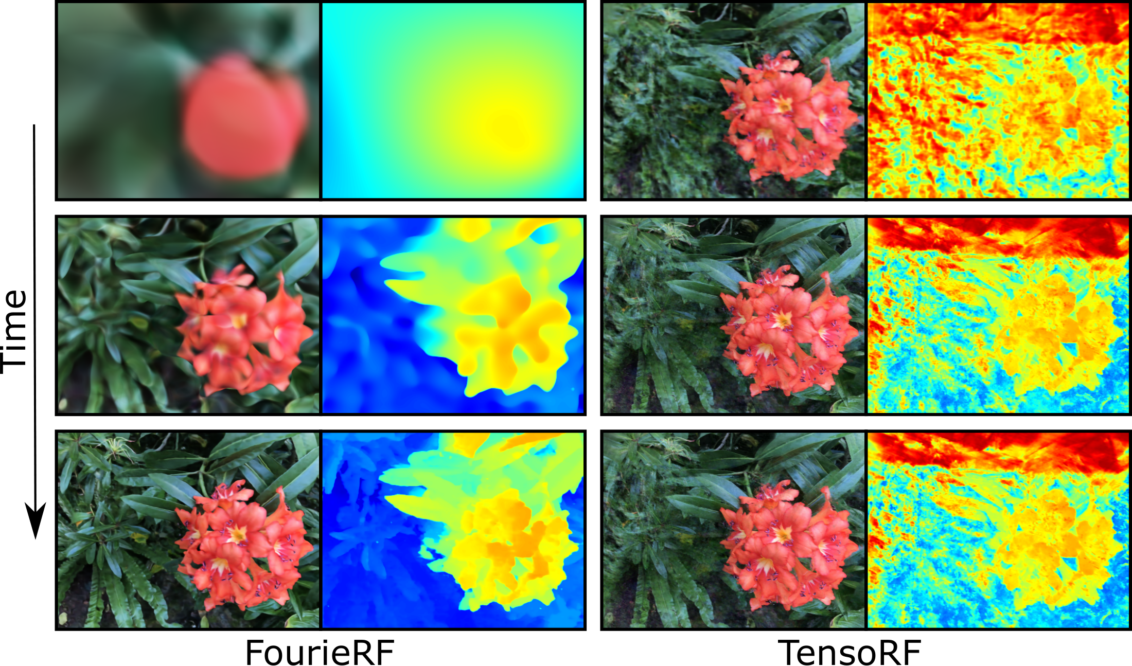
FourieRFPublished

FourieRF: controlling detail from sparse views
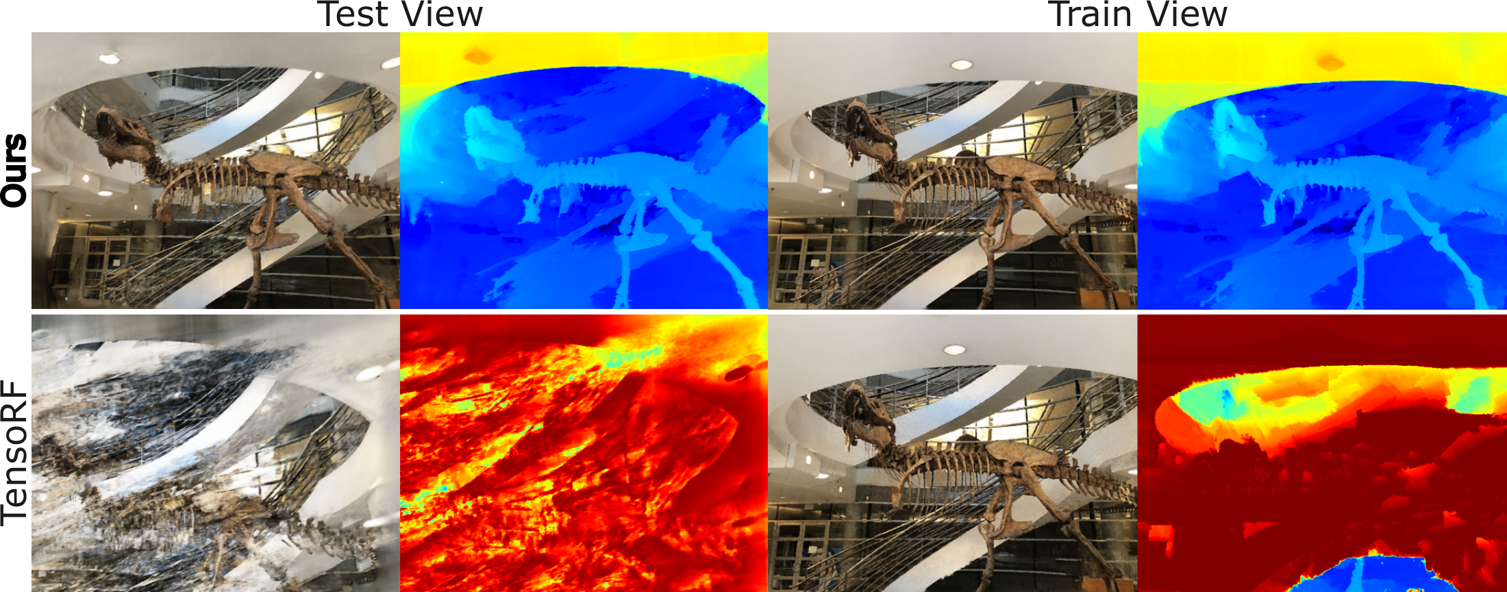
Held-out view on the left; training view on the right. Color and depth reveal different solutions.

Training views can fit well while unseen views fail.

Gomez, Gong & Ovsjanikov · FourieRF · 3DV 20255
FourieRFPublished

Frequency control inside the representation

A compact 3D field sums learned line × plane factors.
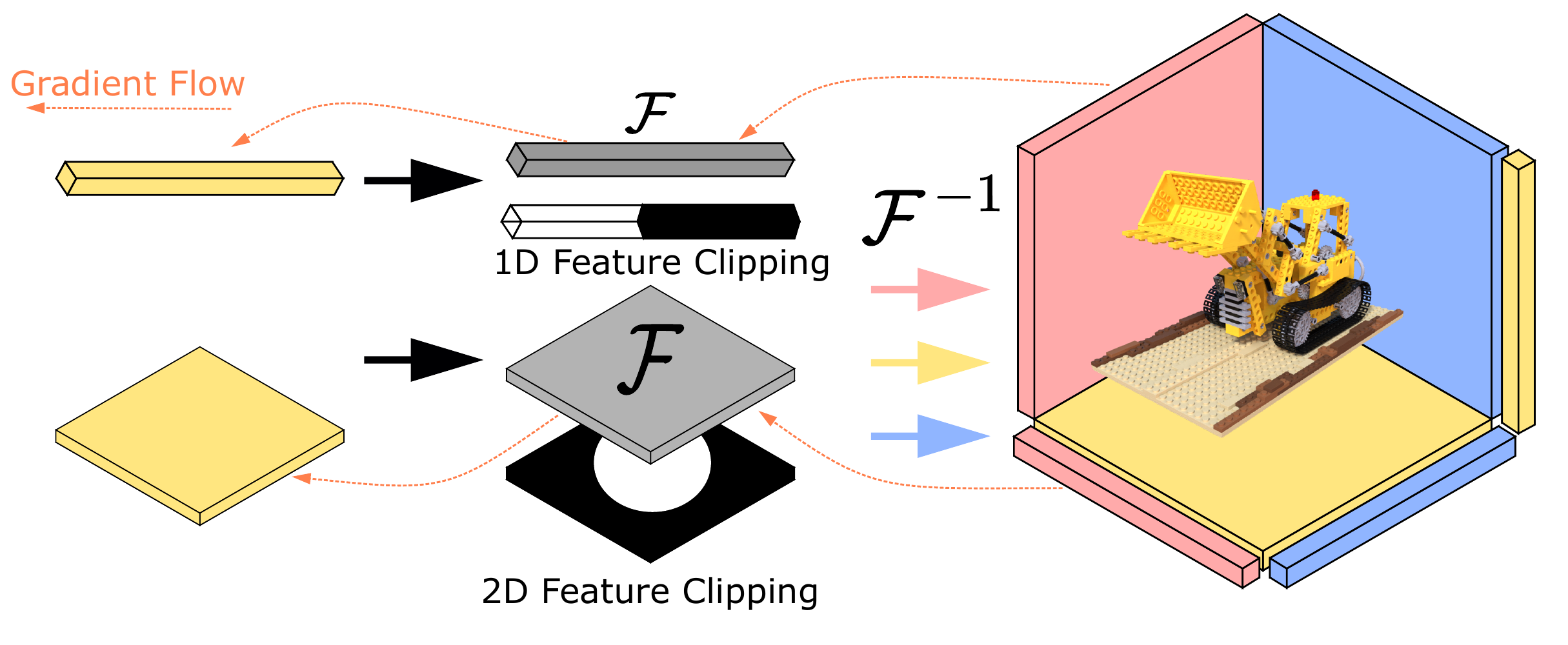
Original FourieRF Figure 2: a learned line and plane are Fourier transformed, clipped by a 1D cutoff or a circular 2D mask, and inverse transformed into smoothed features. Red arrows show gradient flow.
Original method illustration · FourieRF, Fig. 2

1D: frequency cutoff.
2D: centered disk.

bt = bt−1 + Δ

Increase bandwidth
as training progresses.

t = F−1(Mbₜ ⊙ F(f))

Render with the filtered factors; image error trains them through the mask.

Gomez, Gong & Ovsjanikov · FourieRF · 3DV 20256
FourieRFPublished

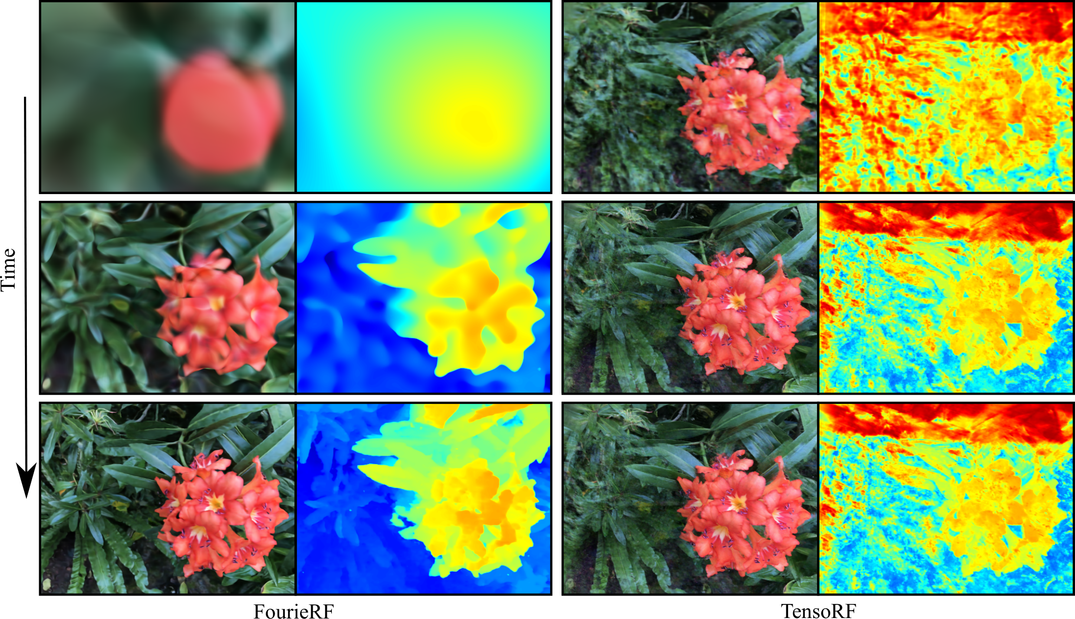
Coarse structure before fine detail

RGB and depth over training, from top to bottom. FourieRF on the left; TensoRF on the right.
Training proceeds downward. Left: FourieRF. Right: TensoRF.

Releasing detail gradually changes the geometry learned from the same images.

Gomez, Gong & Ovsjanikov · FourieRF · 3DV 20257
FourieRFPublished

A measured speed–quality tradeoff

5.57× faster training than ZeroRF,
with 0.212 dB lower PSNR.

MethodRelative training time ↓4-view Blender PSNR ↑
FourieRF-VM0.93021.728 dB
ZeroRF5.18121.940 dB

Reported Blender setup: 10,000 iterations, RTX 4090. Training time normalized to TensoRF = 1.

Frequency control regularizes the field. Geometric use also needs an explicit surface.

Gomez, Gong & Ovsjanikov · FourieRF · 3DV 20258
MILo + SpokesPublished

MILo and Spokes: surfaces from Gaussian splatting

How can Gaussians fitted to images describe a usable surface?

MILo · TOG / SIGGRAPH Asia 2025

From Blobs to Spokes · ECCV 2026
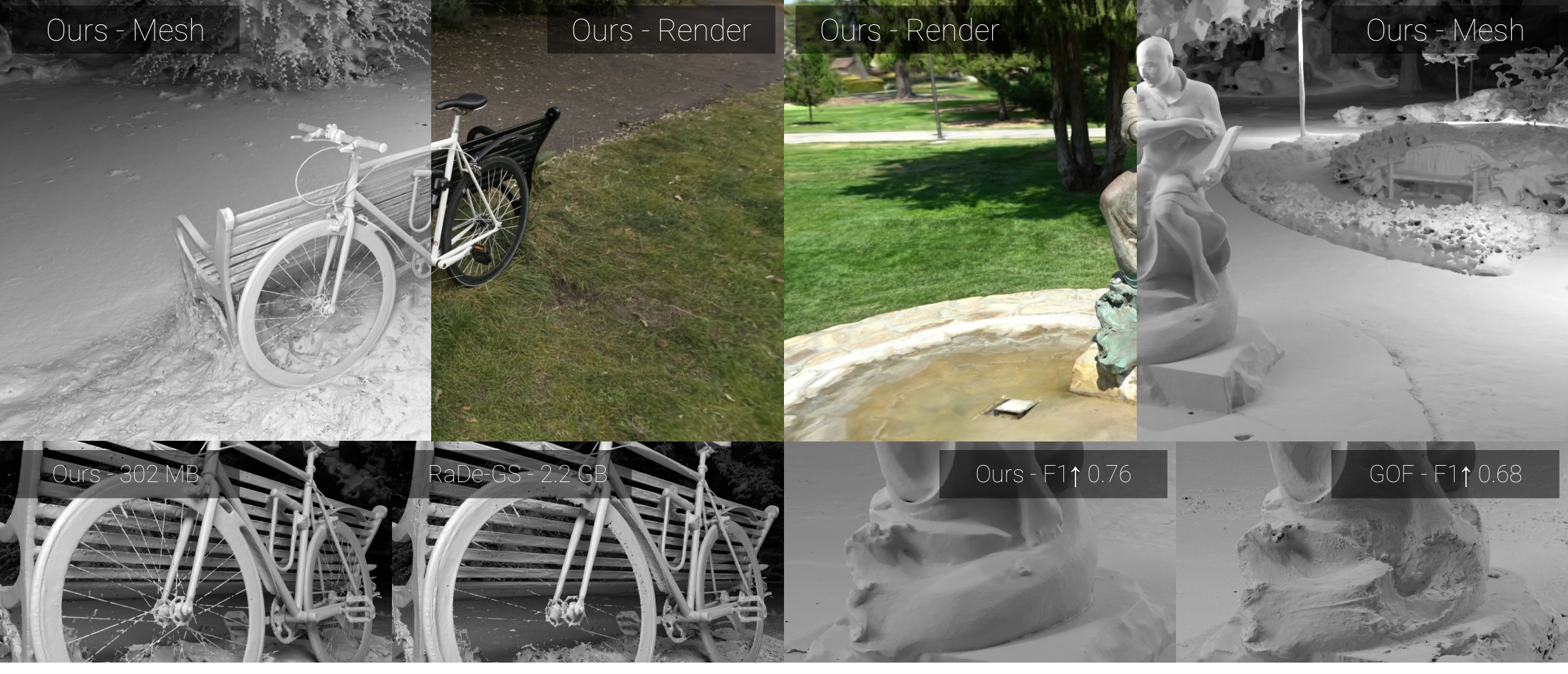
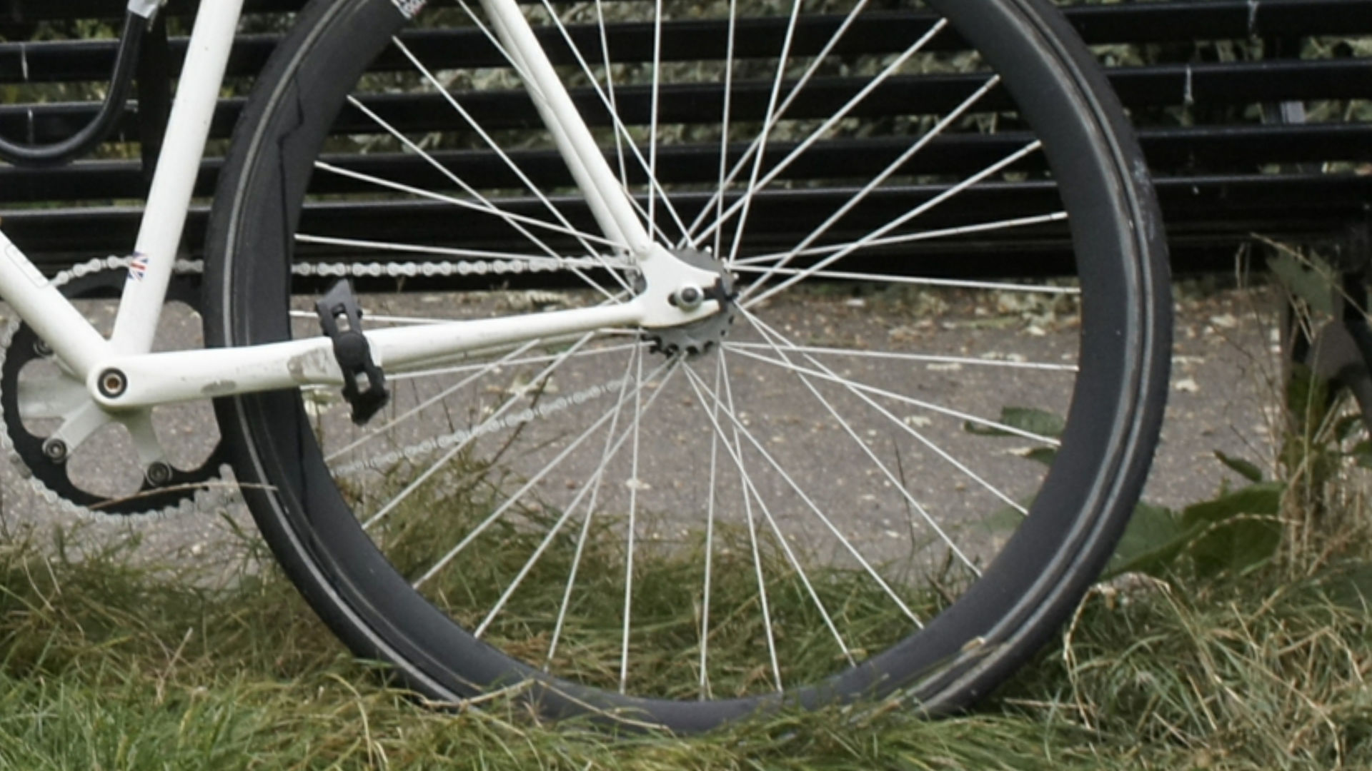
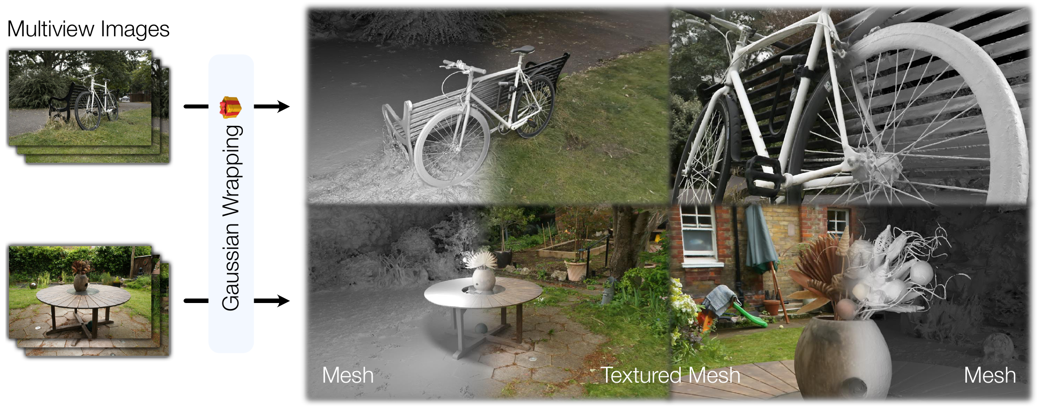
MILo teaser crop: bicycle and bench, with extracted mesh on the left and rendered appearance on the right
Spokes teaser crop: reconstructed bicycle and garden scenes with detailed wheel spokes and plant geometry; multiview input diagram omitted

Let the extracted mesh
constrain training.

Give each Gaussian
an outward surface orientation.

MILo · Guédon et al., TOG 2025 | From Blobs to Spokes · Gomez et al., ECCV 20269
MILo + SpokesPublished

MILo: the extracted mesh constrains training
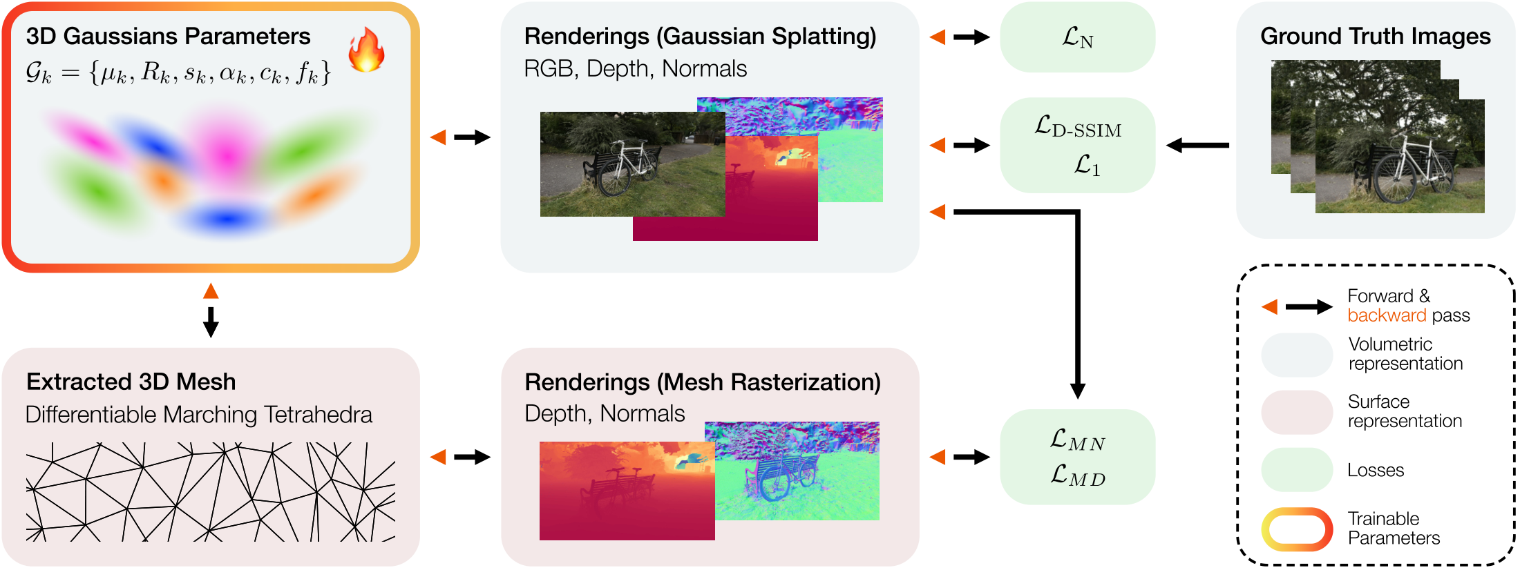
Gaussian rendering and extracted mesh rendering linked by depth and normal losses
The same cameras render both representations. Mesh losses update the parameters that produce the surface.

ℒ = vol + mesh + ℒreg

Image fitting and Gaussian normals + mesh depth/normal agreement + surface regularization

Guédon, Gomez, Maruani, Gong, Drettakis & Ovsjanikov · MILo · TOG 202510
MILo + SpokesPublished

MILo: surface vertices follow the Gaussians
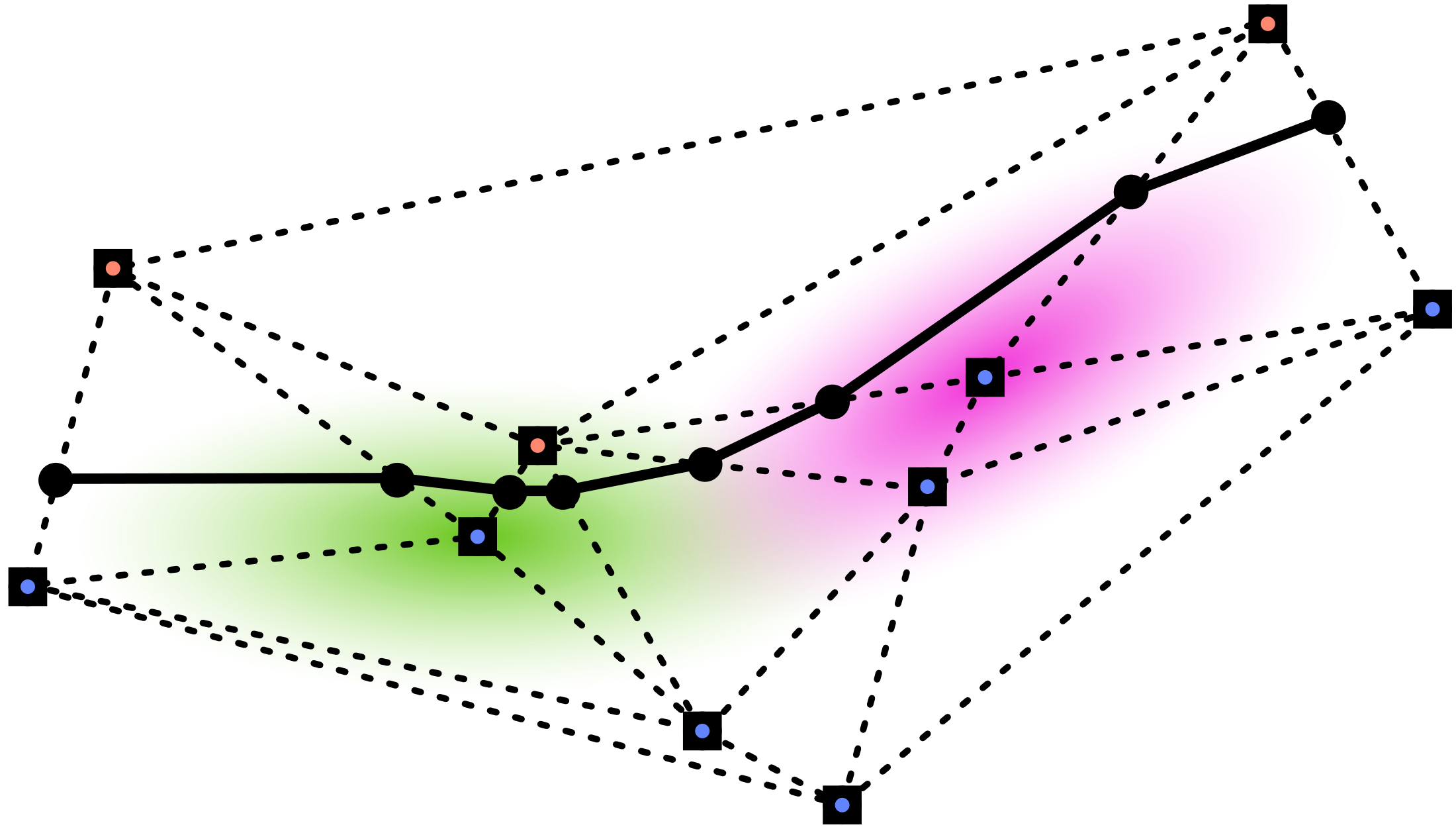
Original 2D schematic of Gaussian-aligned pivots with signed scalar values
Nine pivots in 3D: the Gaussian center and eight aligned box corners.

pk,i = μk + Rk(sk ⊙ bi)

Position μ, rotation R and scale s place each pivot p.
bi: unit-box center or corner.

A learned scalar f marks each pivot as inside or outside.

v = (fₐpᵦ − fᵦpₐ) / (fₐ − fᵦ)

Opposite signs locate the zero crossing: a mesh vertex v.

Mesh losses update both the signed values and the Gaussian geometry.

Guédon, Gomez, Maruani, Gong, Drettakis & Ovsjanikov · MILo · TOG 202511
MILo + SpokesPublished

MILo: depth and normals align volume and surface
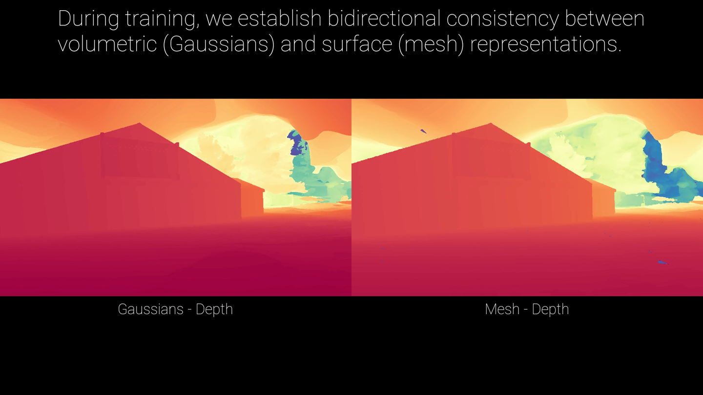
Gaussian and mesh depth and normal renderings during training
Gaussian and mesh renderings from the same camera

Depth locates the visible surface

MD = ∑i log(1 + |D(i) − DM(i)|)

D: Gaussian depth · DM: mesh depth

Normals align its orientation

MN = ∑i [1 − Ñ(i) · NM(i)]

Ñ: normal from Gaussian depth
NM: rasterized mesh-face normal · i: pixel

mesh = λMDMD + λMNMN. Both renderings should describe the same surface.

Guédon, Gomez, Maruani, Gong, Drettakis & Ovsjanikov · MILo · TOG 202512
MILo + SpokesPublished

Spokes: oriented Gaussians define a surface boundary

Learn outward normals; encourage the Gaussians to wrap the surface.
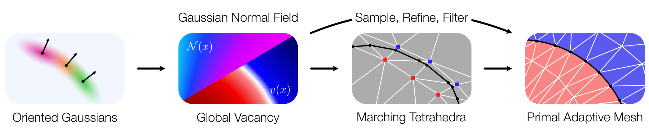
Original Spokes method diagram: oriented Gaussians define normal and vacancy estimates for tetrahedral extraction and optional Primal Adaptive Meshing
Original method figure: normal and vacancy estimates support extraction.

Surface fields

Normal estimates describe orientation.
Vacancy estimates distinguish outside from inside.

Mesh extraction

Two pivots per Gaussian locate the boundary.
Optional PAM adapts mesh resolution.

MILo learns signed values on pivots. Spokes derives fields from oriented Gaussians.

Gomez*, Guédon*, Maruani, Gong & Ovsjanikov · From Blobs to Spokes · ECCV 2026 · * Equal contribution13
MILo + SpokesPublished

Thin structures reveal the difference

Input photograph of the bicycle wheel
Input photograph
MILo reconstruction of the same bicycle wheel
MILo
Gaussian Wrapping reconstruction with finer bicycle spokes
Spokes / Gaussian Wrapping

Bicycle scene: input photograph and surface-normal visualizations.

Oriented Gaussian wrapping recovers more of the wheel’s thin spokes in this example.

Gomez*, Guédon*, Maruani, Gong & Ovsjanikov · From Blobs to Spokes · ECCV 2026 · * Equal contribution14
MILo + SpokesPublished

Mesh complexity and surface accuracy

Surface sampling evaluates geometry independently of vertex density.

MethodMesh vertices ↓
Mesh-rendering evaluation
Uniform F1 ↑Virtual-scan F1 ↑
GOF11.63 M0.310.38
RaDe-GS10.06 M0.350.39
MILo4.36 M0.340.42
Spokes5.80 M0.480.53

Tanks & Temples. Vertices: mesh-rendering evaluation (Table 2). F1: six-scene surface evaluation (Table 1); Spokes F1 uses two pivots, without PAM.

MILo has the fewest reported vertices; Spokes has the highest F1 among these methods.

Gomez*, Guédon*, Maruani, Gong & Ovsjanikov · From Blobs to Spokes · ECCV 2026 · Tables 1–215
Reconstruction → semanticsPublished

Usable geometry still needs semantic handles
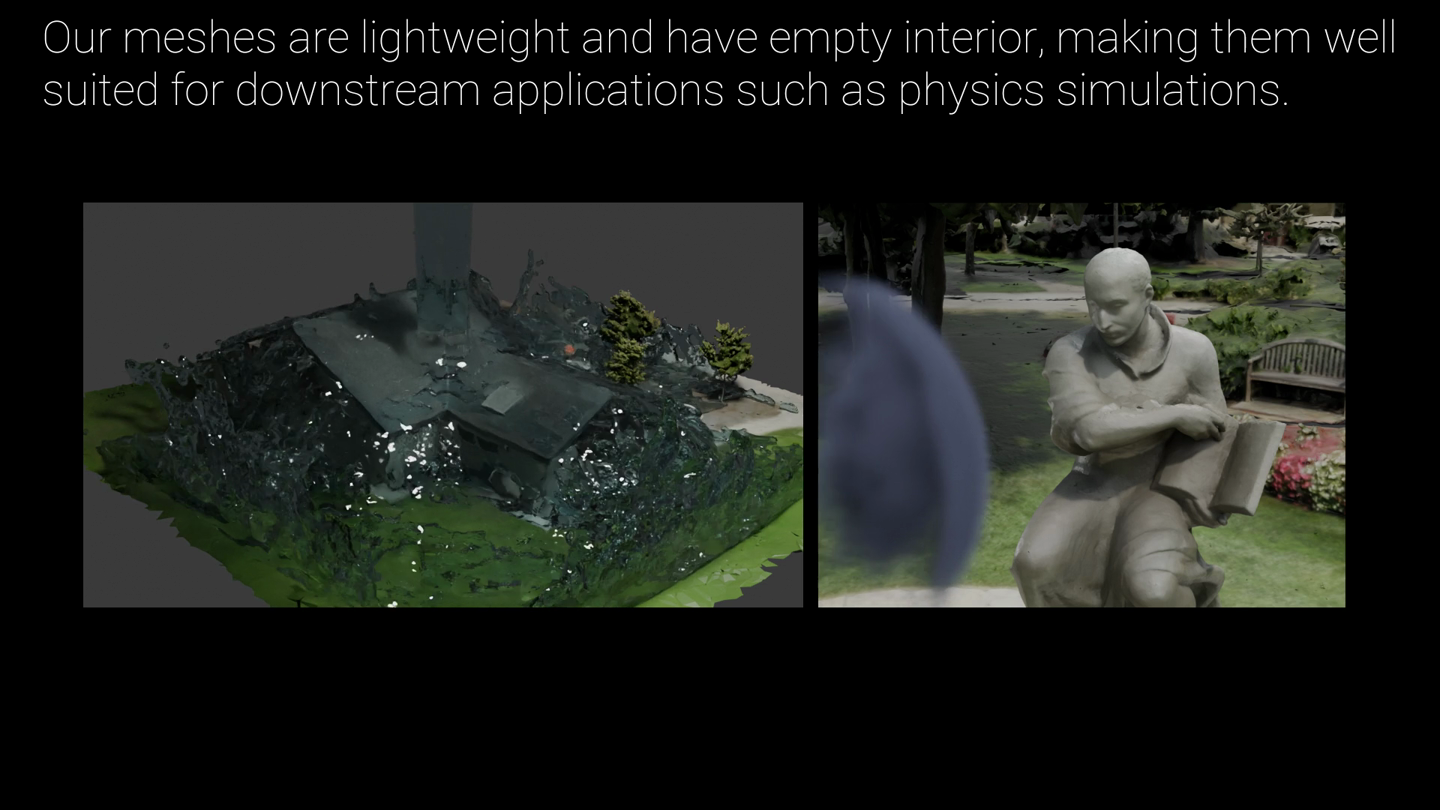
MILo meshes used in downstream simulation.

A surface can support interaction.

But geometry alone does not identify a hinge, a wingtip, or the part a user wants to edit.

The next question is how language can locate meaningful structure.

Guédon, Gomez, Maruani, Gong, Drettakis & Ovsjanikov · MILo · TOG 202516
ZeroKeyPublished

ZeroKey: connecting names to 3D points

Locate named 3D points through agreement across rendered views.
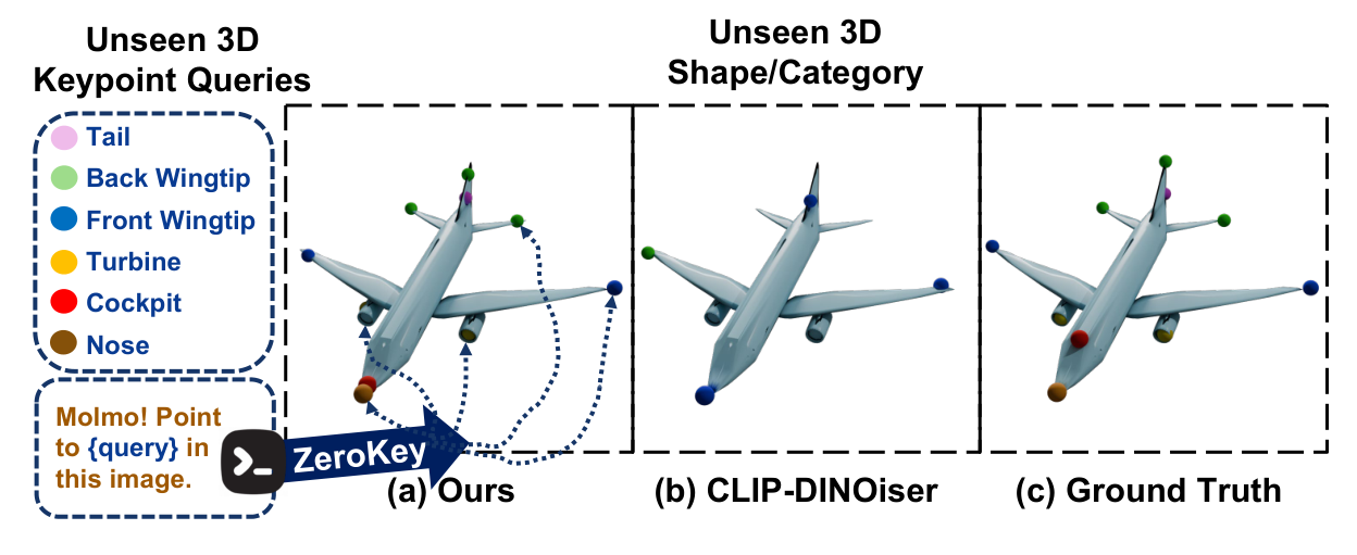
ZeroKey locates named keypoints on an unseen airplane mesh

Query pretrained image models on a known mesh.
Zero-shot: no task-specific 3D keypoint training.

Bingchen Gong, Diego Gomez, Abdullah Hamdi, Abdelrahman Eldesokey,
Ahmed Abdelreheem, Peter Wonka and Maks Ovsjanikov

Gong et al. · ZeroKey · ICCV 202517
ZeroKeyPublished

Language queries become 3D point hypotheses
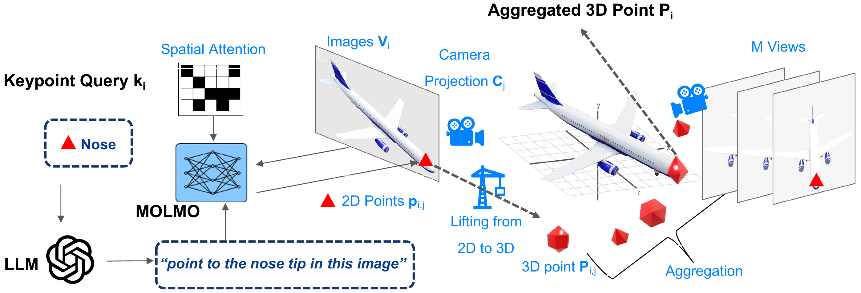
Original ZeroKey pipeline: a text query produces 2D points in rendered views, which are lifted and aggregated in 3D

Language → pixels
GPT-4o proposes names.
Molmo points in 26 rendered views.

Pixels → 3D hypotheses

xj = πj−1(uj, Dj(uj))

uj: predicted pixel; xj: 3D candidate.
Known camera πj; cached mesh depth Dj.

The mesh supplies geometry; the model supplies the point’s meaning.

Gong et al. · ZeroKey · ICCV 202518
ZeroKeyPublished

A name selects the target; 3D agreement stabilizes it
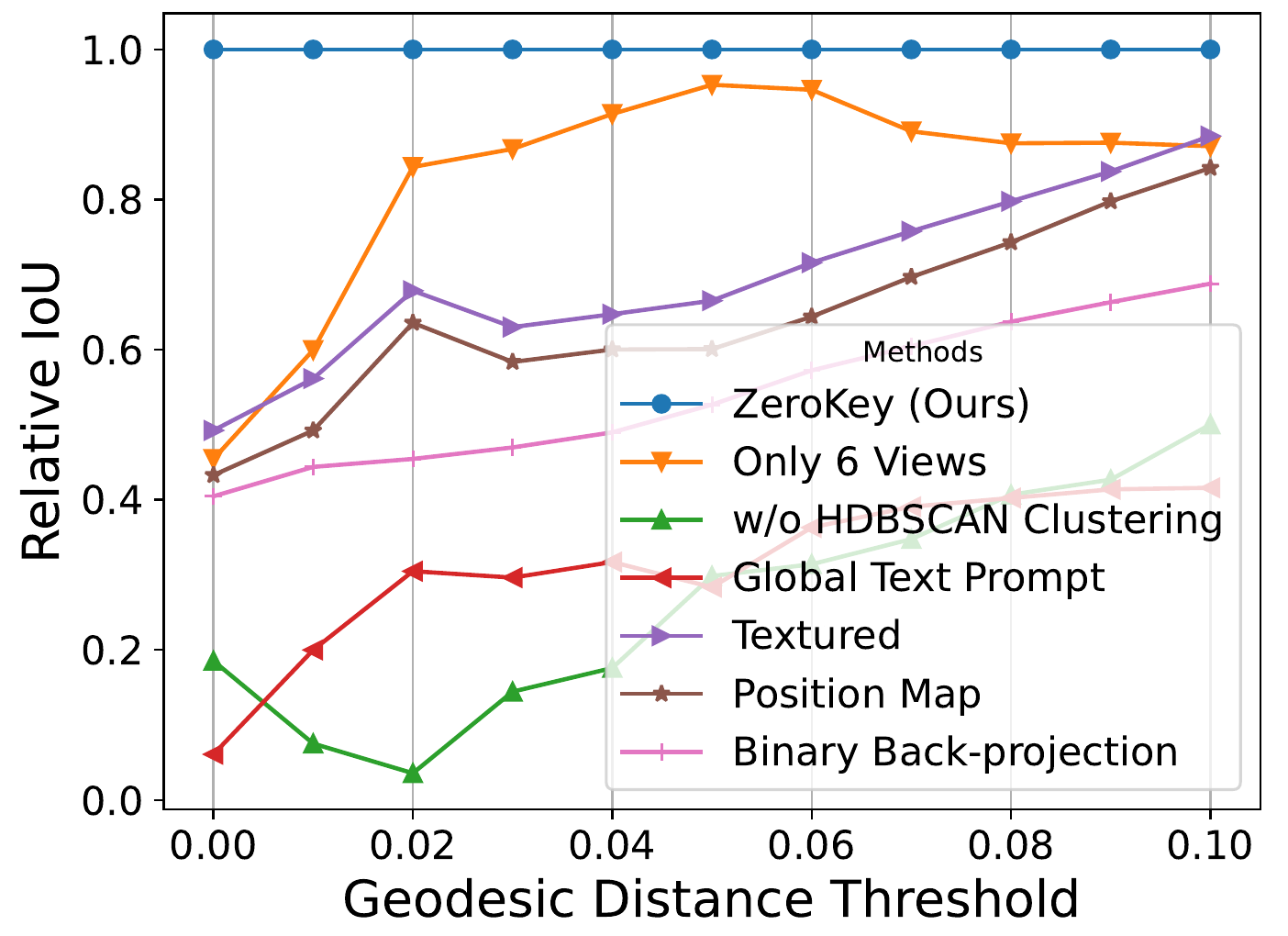
Original ablation plot: relative IoU for specific versus global prompts, soft versus binary back-projection and HDBSCAN versus direct averaging
Relative IoU; full ZeroKey = 1 at each threshold.

Local uncertainty
Lift an h × h neighborhood; use Gaussian support weights.

Agreement in 3D
HDBSCAN separates consistent groups and rejects isolated detections.

One name can denote several corners. Preserve separate spatial hypotheses.

Global prompts, binary weights and direct averaging all reduce performance in this experiment.

Gong et al. · ZeroKey · ICCV 202519
ZeroKeyPublished

Semantic grounding still leaves a precision gap

KeypointNet: airplane, chair and table. IoU (%) at geodesic distance thresholds.

Method0.010.050.10
GPT-4o localizer0.486.0420.73
B2-3D · few-shot, 62 views20.2957.7270.57
ZeroKey · 26 views13.1656.6079.43

Benchmark queries are human-written descriptions of keypoint IDs.
ZeroKey requires no task-specific 3D keypoint training.

Names help identify the intended structure; tight tolerances expose localization errors.

Gong et al. · ZeroKey · ICCV 2025 · Table 120
ZeroKeyPublished

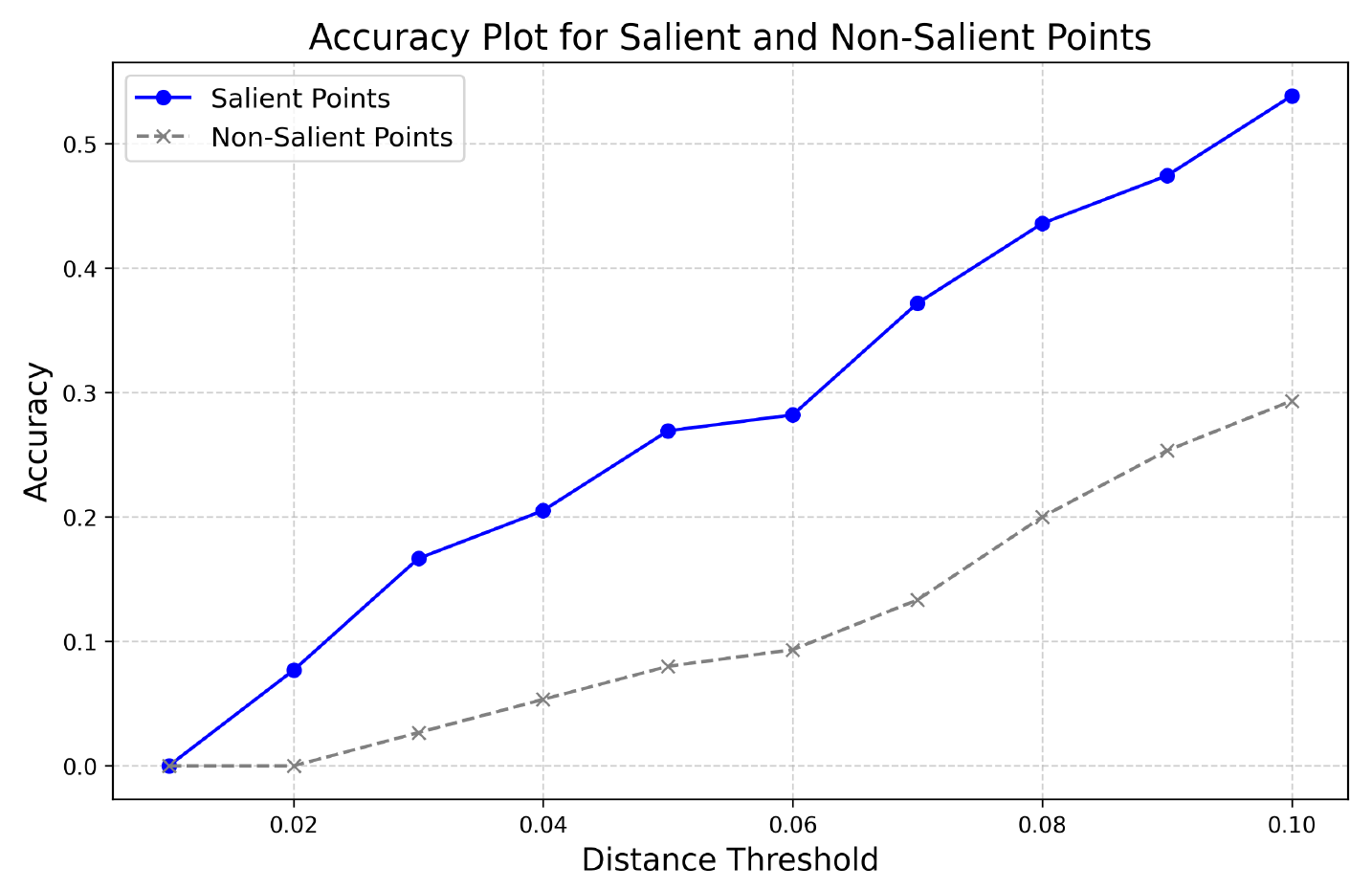
Can language recover the point it describes?

Nameability test: marked point p → short description ℓ → recovered point p̂
Keep the most repeated description; query new views with the marker removed.
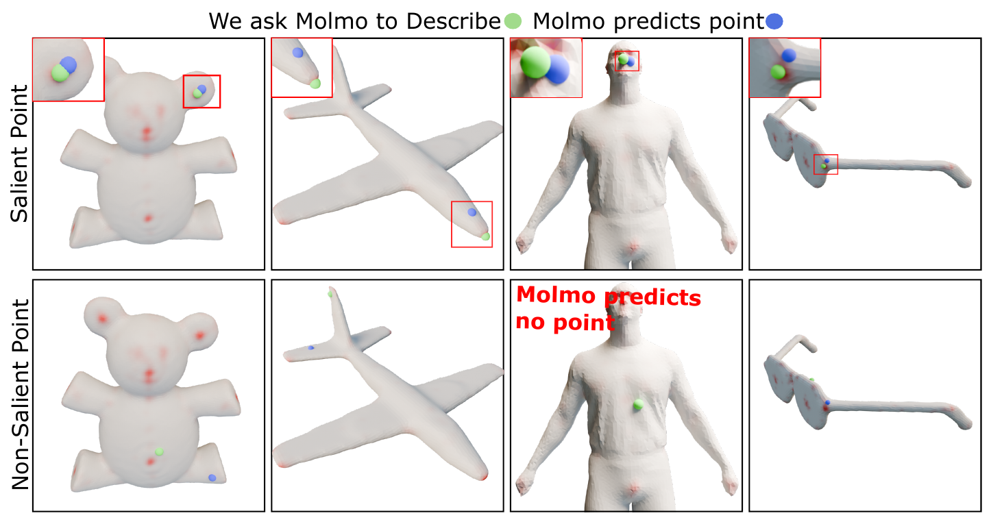
Original salient and non-salient examples: describe the green marked point and retrieve the blue point; some arbitrary points yield no prediction
Human saliency: Schelling-point selection density.
Original retrieval-accuracy plot: salient points are more accurately recovered than non-salient points across the tested absolute 3D error thresholds
Retrieval stability: recovery within a 3D error tolerance.

Human-salient points are easier to recover from their descriptions.

Interpretation: distinctive names can give 3D points shared, repeatable identities.

Gong et al. · ZeroKey · ICCV 2025 · Figures 4–5; supplement Algorithm 121
PatchAlign3DPublished

PatchAlign3D: language-aligned local features

Encode the shape once; query regions with part names.
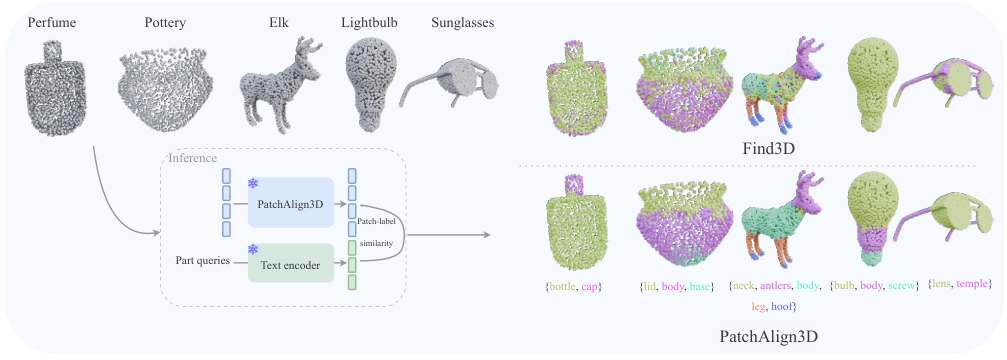
Point-cloud features compared with text-defined parts
A trained 3D encoder matches local features to text embeddings.

Several part names can describe the same patch.

Souhail Hadgi, Bingchen Gong, Ramana Sundararaman, Emery Pierson,
Lei Li, Peter Wonka and Maks Ovsjanikov

Hadgi et al., PatchAlign3D, CVPR 202622
PatchAlign3DPublished

Visual distillation, then local language alignment
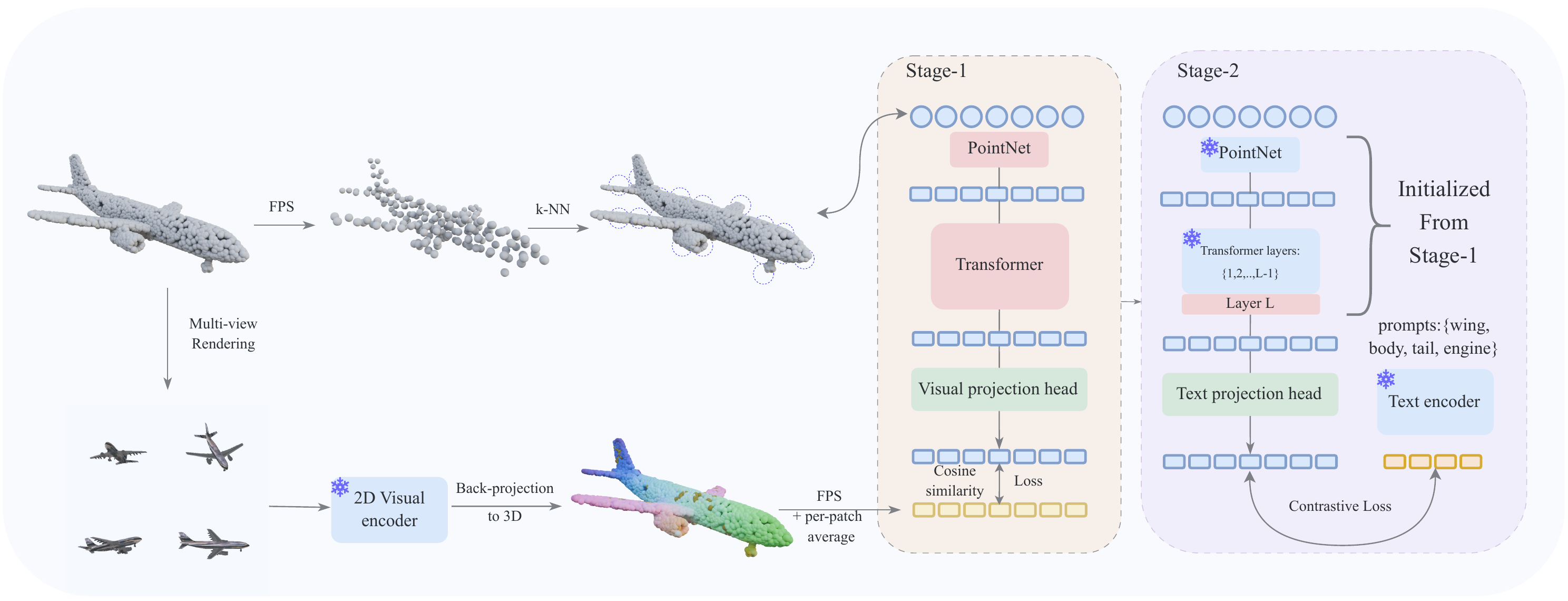
Original PatchAlign3D training pipeline, with frozen visual and text encoders and the trainable last transformer block highlighted
2,048 XYZ points · 128 overlapping patches of 32 points · 12 transformer blocks

Stage 1 · visual structure
Match 3D patch features to frozen DINOv2 targets
with a cosine loss.

Stage 2 · language alignment
Freeze the first 11 blocks; train the last block
and projection into OpenCLIP’s text space.

Hadgi et al. · PatchAlign3D · CVPR 202623
PatchAlign3DPublished

A patch can match several part descriptions

Training labels: 10 rendered views → SAM regions → Gemini part names → 3D pseudo-labels.

Fractional target yij
Share of patch i annotated with name j.

NameAnnotated pointsyij
Nose24 / 320.75
Muzzle32 / 321.00
Ear0 / 320.00

Illustrative patch with overlapping annotations.
The targets need not sum to one.

“Nose” and “muzzle” can both be valid positives.
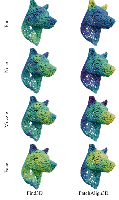
Original text-similarity maps for ear, nose, muzzle and face: Find3D compared with PatchAlign3D
Text-similarity maps; yellow means higher similarity.
Hadgi et al. · PatchAlign3D · CVPR 202624
PatchAlign3DPublished

Contrastive learning needs the right negatives

sij = ⟨qi, tj⟩ / τ + b,   pij = sigmoid(sij)

Ltext = −∑i,j [yij log pij + (1 − yij) log(1 − pij)]

qi = htext(zi): projected patch feature; tj: text embedding; τ: learned temperature; b: learned bias.

Independent patch–text pairs
Sigmoid allows several positive names.

Negatives within each shape
Use its valid part names with yij = 0.

ShapeNetPart · mIoU (%)

Negative samplingmIoU
Within shape56.9
Also across shapes45.3

A “leg” on another shape may be a false negative, not a different concept.

Hadgi et al. · PatchAlign3D · arXiv v2 · Equations 4–5; supplement Table 1225
PatchAlign3DPublished

Visual structure first, language alignment second
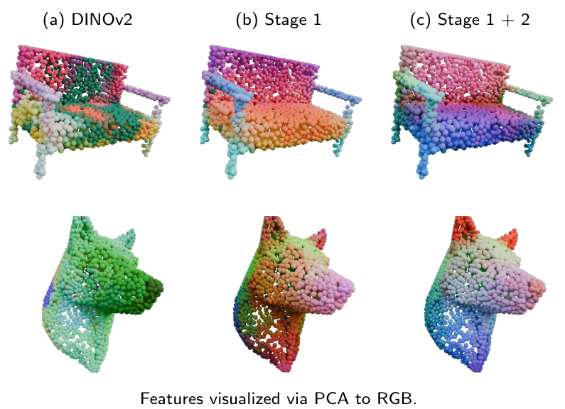
DINOv2, Stage 1 and Stage 1 plus Stage 2 local features visualized with independent PCA
Independent PCA projections; colors do not match across columns.

Training order matters

ShapeNetPart · mIoU (%)

TrainingmIoU
Language alignment only50.5
Both losses jointly50.2
Visual → language56.9

Preserve local visual structure while learning what its regions are called.

Point-cloud baselines: COPS 25.6; Find3D 23.3 mIoU. Reported runtime: PatchAlign3D and Find3D both 0.4 s/shape.

Hadgi et al. · PatchAlign3D · CVPR 202626
PatchAlign3DPublished

Patch features can support ZeroKey’s point proposals

Semantic support for voting
Use patch–text similarity to modulate ZeroKey’s soft-voting weights.

Local features for clustering
Add learned feature cues when grouping the 3D point proposals.

Reported KeypointNet comparison · IoU (%) at geodesic distance thresholds

Method0.010.050.10
ZeroKey13.1656.6079.43
PatchAlign3D + ZeroKey10.4258.8781.27

IoU improves at 0.05 and 0.10, but falls at 0.01.

The hybrid still uses ZeroKey’s multiview pipeline.

Hadgi et al. · PatchAlign3D · arXiv v2 · Supplement C, Table 1427
Learning from feedbackOngoing work

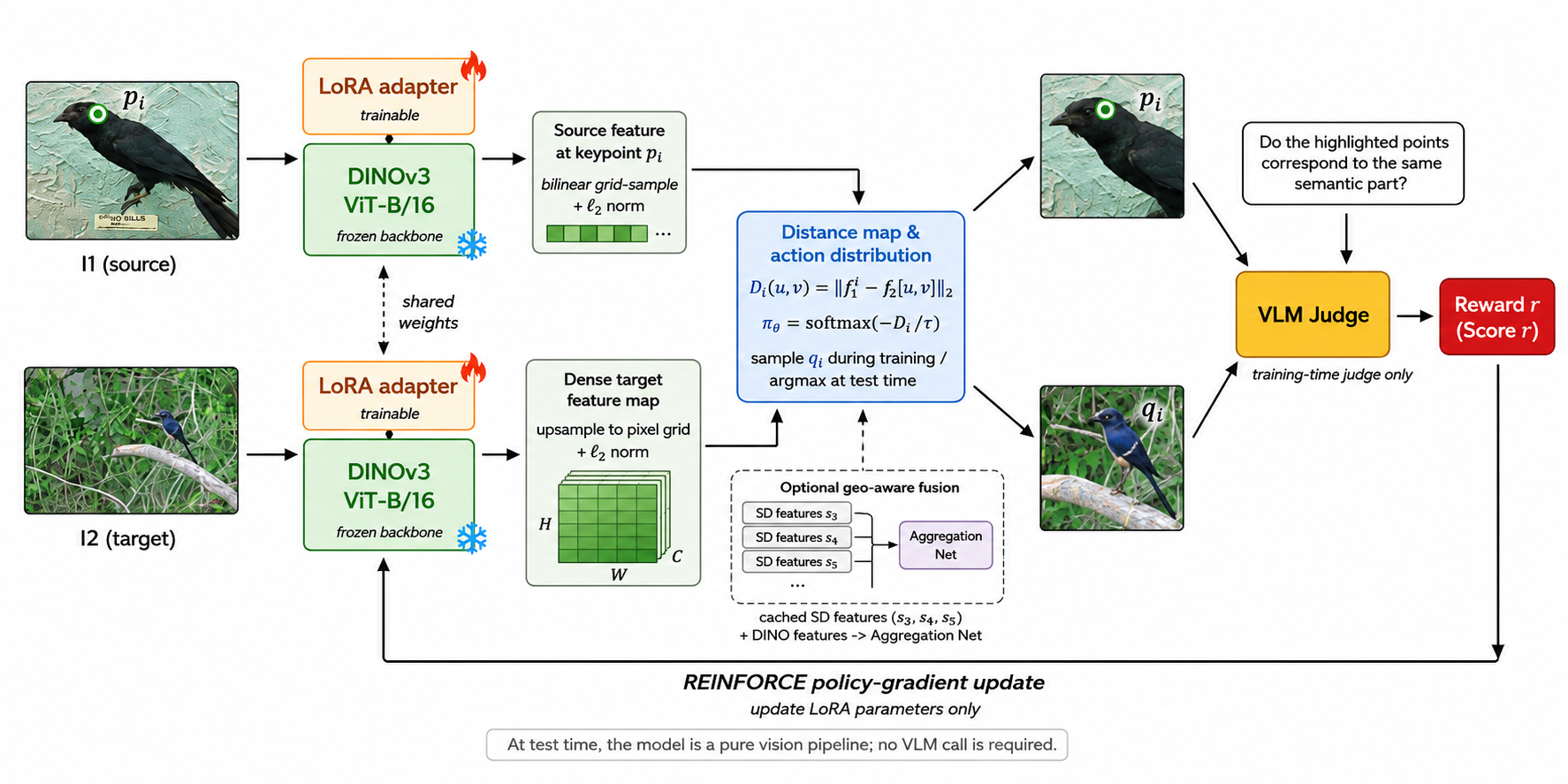
Is It a Good Match? A VLM as the training judge

Given two images and a source point, learn its target match.

Image pair + pointGiven I₁, I₂ and pDINOv3 + LoRASample target pixel qFrozen VLMScore the marked pairREINFORCEUpdate LoRAReward relative to the baseline changes the sampled match’s probability

ZeroKey
Query an image model for points during inference.

Good Match
Judge visual proposals during training; infer without a VLM.

Bingchen Gong · Viktoria Ehm · Emery Pierson · Maks Ovsjanikov

Gong, Ehm, Pierson & Ovsjanikov · Is It a Good Match? · ongoing work28
Learning from feedbackOngoing work

A one-step policy over target pixels

Context sImages I₁, I₂ and source point p
Action qOne sampled target pixel
Reward r ∈ [0, 1]“Same semantic part?”A frozen VLM scores the marked pair.

Feature distance → policy

D(q) = ‖f₁(p) − f₂(q)‖₂

πθ(q | s) = exp(−D(q)/τ) / Σq′ exp(−D(q′)/τ)

Shared encoder: f₁ = gθ(I₁), f₂ = gθ(I₂).
τ = 0.1 controls sampling diversity.

Adapt only the LoRA weights

W′ = W + (α / rL) BA

W stays frozen. A and B learn.
Low-rank updates to ViT Q/K/V projections.

LoRA rank rL = 16; scale α = 8.

Train: sample q ∼ πθ. Test: take argmaxq πθ(q | s), without a judge.

Gong, Ehm, Pierson & Ovsjanikov · Is It a Good Match? · ongoing work29
Learning from feedbackOngoing work

REINFORCE learns from a non-differentiable score

Reward above the recent baseline reinforces the sampled match.

t = −(1/B) (rt − bt) log πθ(qt | st)

Advantage: rt − bt

Frozen judge returns rt ∈ [0, 1].
Use bt before adding the current reward.

bt+1 = 0.99 bt + 0.01 rt

Accumulate B = 10 samples per update.

Gradient through the policy

Differentiate log π through the adapter.
Hold reward and baseline fixed.

Positive advantage: increase probability.
Negative advantage: decrease probability.

Keep valid zero scores; skip invalid responses.

No gradient through the VLM; no target-coordinate annotation in the reward.

Gong, Ehm, Pierson & Ovsjanikov · Is It a Good Match? · ongoing work30
Learning from feedbackOngoing work

VLM reward improves matching across 18 categories

SPair-71k, all 18 categories · Peak validation PCK@bbox 0.10 (%)

MethodPCK ↑
Frozen DINOv354.20
DINOv3 + LoRA67.83
Geometry-aware + LoRA71.20

Both trained models use REINFORCE
with Gemini Pro reward.

+13.63PCK points
LoRA adaptation
+17.00PCK points
with geometry-aware features

Both gains are relative to frozen DINOv3.

Training and evaluation span the same 18 categories.

Source points are given. Target-coordinate labels do not enter the reward.

Gong, Ehm, Pierson & Ovsjanikov · Is It a Good Match? · ongoing work31
Learning from feedbackOngoing work

Reward precision and geometric feedback

Right part ≠ exact location

Qwen3-VL-32B-Thinking scores plateau within ≈20 px in a 126-keypoint cat probe.

Separate calibration probe with a different judge.

Separate cat-only transfer test
Cat-trained plain LoRA gains only +0.02 mean PCK across six other categories.

The 3D pilots do not establish successful transfer.

What changes under feedback?

Good Match · training
Propose a match → score → update visual weights.

3DHarness · inference
Execute a program → inspect renders or measurements → revise the program.

Feedback must distinguish the geometric errors the task needs to correct.

Gong, Ehm, Pierson & Ovsjanikov · Is It a Good Match? · ongoing work32
Executable 3D hypothesesOngoing work

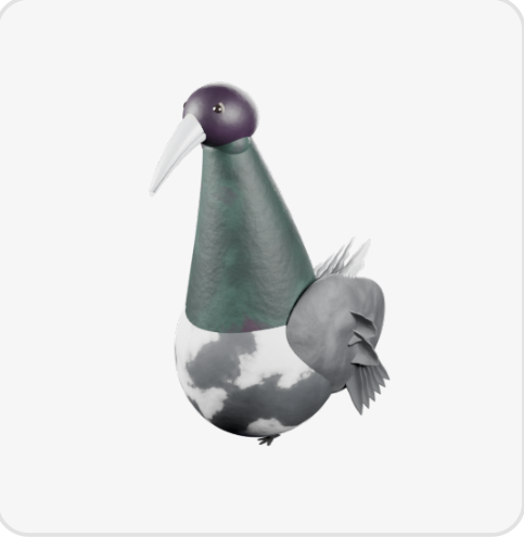
3DHarnessBench: a program as a 3D hypothesis

What does the agent believe
the object is made of?

  • Parts and their dimensions
  • Transforms, symmetry and repetition
  • Geometry and material procedures

Ling Liu · Bingchen Gong
Amal Dev Parakkat · Maks Ovsjanikov

P  →  E(P) = Ĝ

Blender Python  →  Executed 3D object
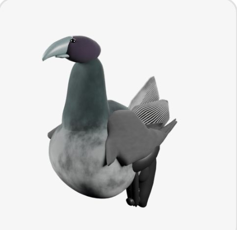
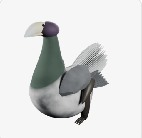
Bird reconstructed by an executable Opus 5 program

Execution makes the inferred structure observable and measurable.

100 targets from 3DCodeBench, one per category. Original source programs are withheld.

Liu, Gong, Parakkat & Ovsjanikov · 3DHarnessBench · ongoing work33
Executable 3D hypothesesOngoing work

Code expresses repetition, symmetry and named parts

Target
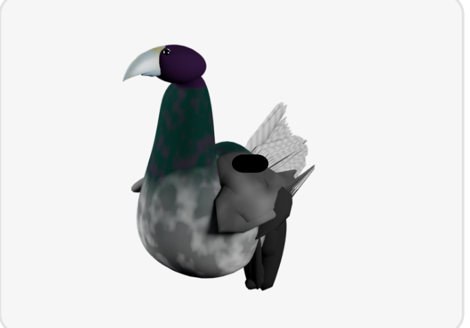
Target bird

Excerpts from the generated Blender Python

Repeat feathers along a row

for i in range(n):
    s = i / float(n - 1)

Mirror the wing geometry

wf.mirror_y()

Create a named component

wf.object(PFX + "wing_feathers")

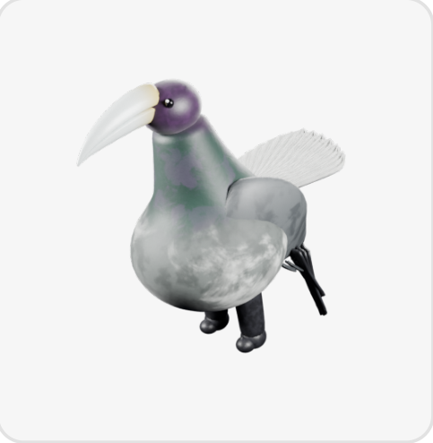
Result

Opus 5 reconstruction under Full 3D Interaction

Construction rules become explicit operations the agent can revise.

Opus 5, Full 3D Interaction. Placement calculations and coordinate tables omitted.

Liu, Gong, Parakkat & Ovsjanikov · 3DHarnessBench · ongoing work34
Executable 3D hypothesesOngoing work

Observe, write, execute, inspect and revise

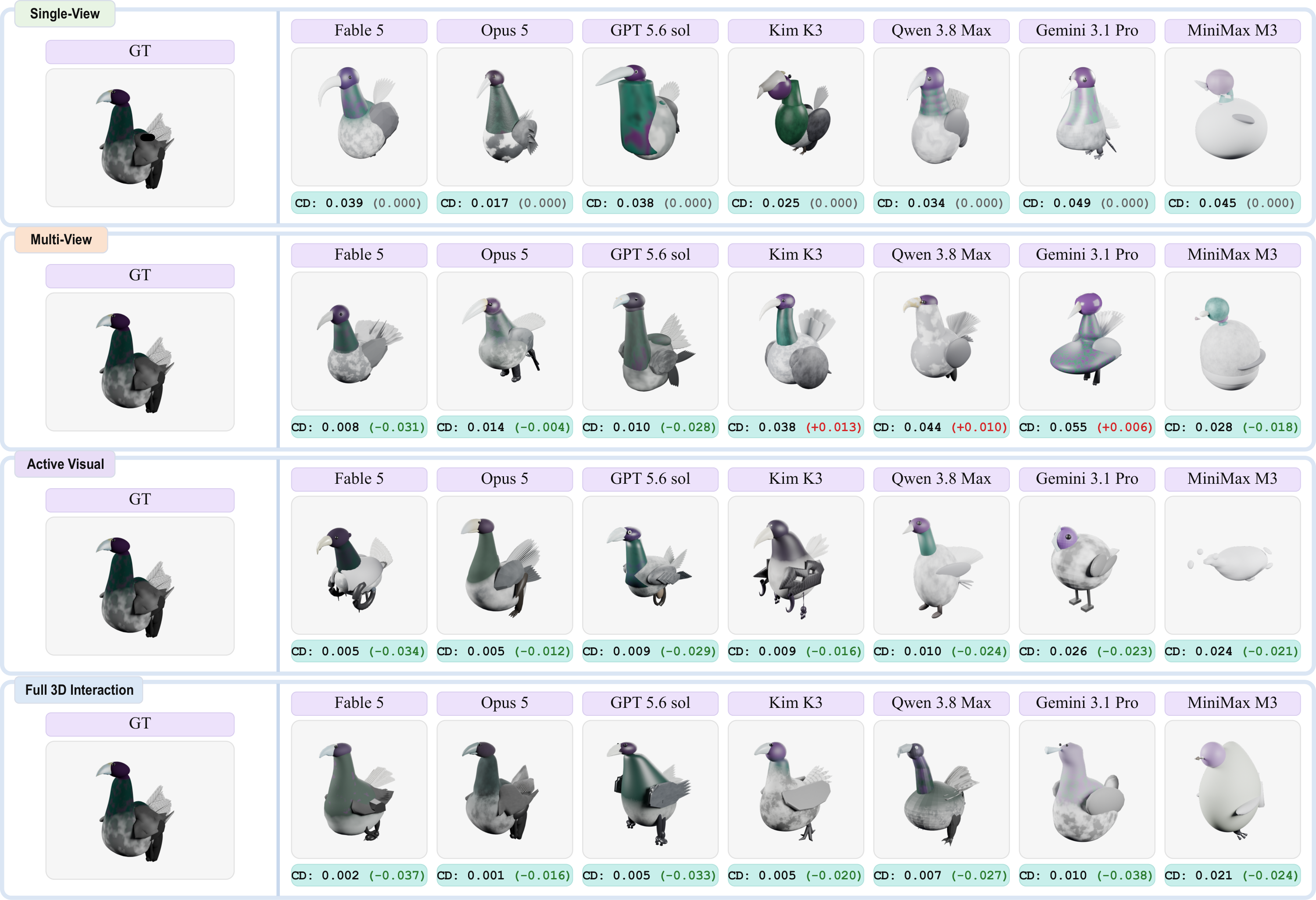
Single viewOne fixed imagePassive observationMulti-viewFour fixed imagesPassive observationActive visualAgent chooses viewsVisual inspection onlyFull 3DViews + measurementsGeometric queriesTarget-side evidenceAcquire evidenceViews or measurementsWrite / revise programExecutable Blender PythonExecute and compareGenerated 3D objectRevise P using evidence from the target and the executed object.
Fixed views: three refinement rounds. Interactive settings: agent-directed tool use.
3DHarnessBench · target-access settings; diagram redrawn from the protocol35
Executable 3D hypothesesOngoing work

Different evidence produces different executable structures

Target

Target bird reconstruction
Reference

Single view

Single view bird reconstruction
CD 0.017

Four fixed views

Four fixed views bird reconstruction
CD 0.014

Active visual

Active visual bird reconstruction
CD 0.005

Full 3D

Full 3D bird reconstruction
CD 0.001

Four separate completed runs. Normalized, rotation-aligned Chamfer ↓ for this object.

Opus 5: richer evidence helps recover proportions, wings and legs.

3DHarnessBench · bird visualization · Opus 5; separate harness runs36
Executable 3D hypothesesOngoing work

Useful observations matter more than access alone

100-target comparison

Agent4 viewsActiveFull 3D
Opus 5.748.871.927
Gemini 3.1 Pro.753.691.783

Uni3D 3D–3D similarity ↑
Active view selection helps one agent and hurts another.

Controlled viewport ablation

.3722  →  .6148

MiniMax Uni3D after normalizing its viewport screenshots.

10 targets, agent still chooses its views.
Four fixed views on this subset: .6200.

Program revision depends on obtaining evidence that reveals what to change.

Liu, Gong, Parakkat & Ovsjanikov · 3DHarnessBench · ongoing work37
Executable 3D hypothesesOngoing work

Measurements constrain the geometry expressed in code

Target evidenceChamfer ↓Uni3D ↑
Images.0150.8133
+ global.0103.8088
+ parts.0099.8557
+ global and parts.0084.8296

10 targets · Opus 5
Fixed multiview input plus measurements

44%lower normalized
Chamfer distance

Global: center, bounds and dimensions.

Parts: anonymous centers, dimensions and repetition statistics.

Parts alone give the best Uni3D.
Combining cues does not improve every metric.

A program can express measured dimensions and relations as construction parameters.

3DHarnessBench · measurement ablation; proposed synthesis38
Executable 3D hypothesesOngoing work

Code provides a state that can be revised and re-executed

First program versus final program

AgentInitialFinal
Opus 5.914.927
Qwen 3.8 Max.796.857
MiniMax M3.566.679

Full 3D · Uni3D ↑ · 100 targets
Larger repair gains need not yield a better final object.

What the representation enables

Inspect a construction choice.
Change a part, parameter or procedure.
Execute again and assess the result.

Next: learn which observation and code revision will fix an error.

Proposed follow-up: train on verified interaction traces and test semantic edits.

This benchmark evaluates reconstruction and interaction. Program quality and semantic editability remain open.

Liu, Gong, Parakkat & Ovsjanikov · 3DHarnessBench · ongoing work39
Research synthesis

Five ingredients, one programme

FourieRF held-out view and depth comparison
Sparse-view geometry
Gaussian surface reconstruction examples from From Blobs to Spokes
Usable surface
ZeroKey semantic point localization examples
Semantic handles
Good Match visual matching and VLM reward pipeline
Learned feedback
3DHarnessBench target and executable reconstruction examples
Executable objects
Research questionUseful structureEvidence or feedback
Reconstruct with limited evidenceControlled feature frequenciesHeld-out views and geometry
Recover a usable surfaceMesh in the loop; oriented GaussiansDepth and normal consistency; debiased surface protocols
Locate meaningful elementsSemantic points and part featuresLocalization and segmentation
Improve a predictorAdapted visual featuresTraining-time model judgments
Construct and repair 3D objectsExecutable programsGeometry, appearance and interaction

The evidence comes from separate projects. The programme tests whether these structures can work together.

Synthesis of the presented research · Programme: From Video to Animatable and Efficient 3D Worlds40
Future programmeProposed work

Articulation exposes testable constraints

“Can the drawer open without hitting the chair?”

  • Identify the moving part and its relation to the frame.
  • Execute the permitted motion.
  • Check contact, collision and appearance consistency.
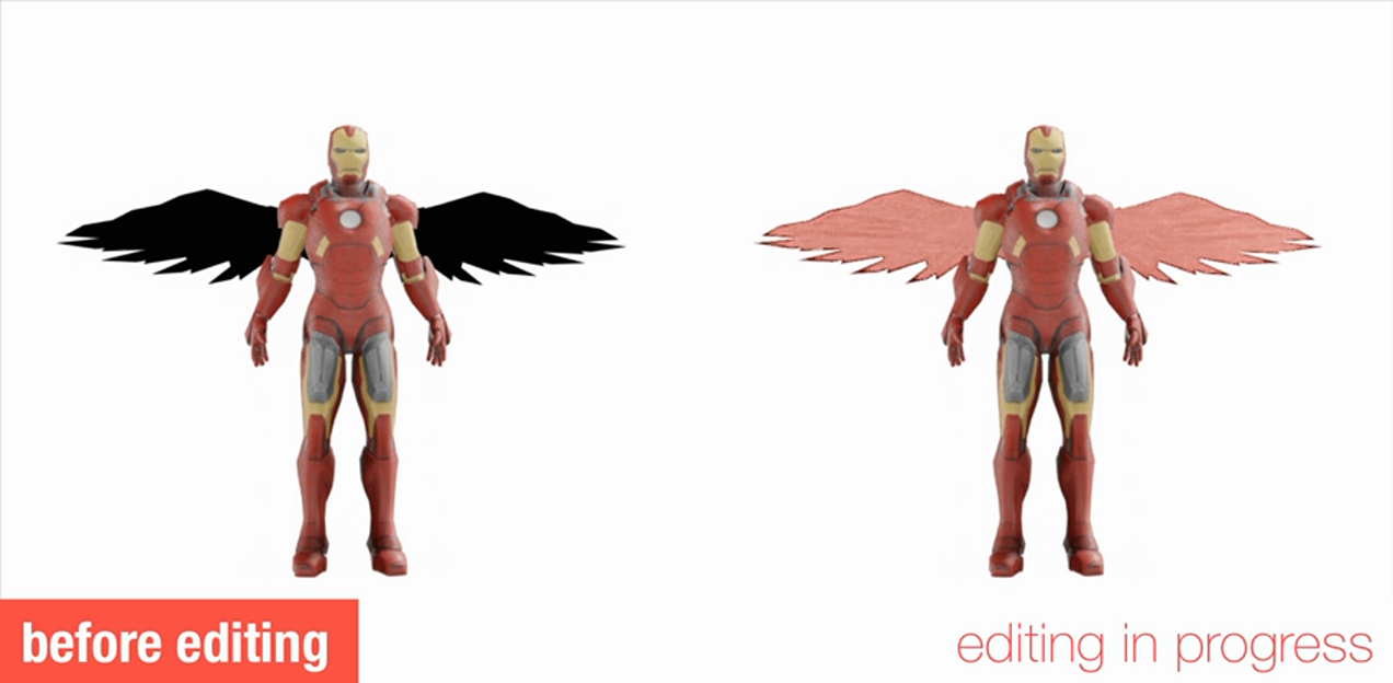
SeamlessNeRF before and during a part composition edit
Prior part composition edit; articulation and collision checks remain proposed.

Conceptual scene description

part: drawer
parent: cabinet
joint: prismatic
axis: local x
range: bounded
constraint: no collision

Illustrative schema for the proposed representation

Télécom Paris research proposal, spatial queries and articulated scenes41
Future programmeProposed work

Explicit structure with neural appearance

Published components motivate a proposed hybrid.

MILo pipeline with Gaussian reconstruction and mesh supervision
Explicit surface
MILo: mesh in the loop
From Blobs to Spokes oriented Gaussian surface extraction
Oriented geometry
Spokes: Gaussian surface field
FourieRF sparse-view reconstruction examples
Neural appearance
FourieRF: image-based detail

These building blocks were studied separately. Their integration is proposed work.

Test the hybrid against pure-program, mesh and Gaussian representations.

Télécom Paris research proposal, Axis 142
Future programmeProposed work

Compact models can learn from verified interaction

Existing evidence shows the two ends of the loop.
3DHarnessBench program revision and executed reconstruction comparison
3DHarnessBench: inference-time observe, revise, execute
Good Match VLM reward and visual feature adaptation pipeline
Good Match: training-time judge and feature adaptation
Verified trajectoriesPrograms, observations and repairs
Compact modelHeld-out edits and task families

The transfer study is proposed. Match information access and compute.

Télécom Paris research proposal, Axis 243
Future programmeProposed benchmark

4DHarnessBench would evaluate operations over time

Proposed tracks, illustrated by prior examples

MILo mesh used in downstream simulation
Articulation
parts, axes and motion
SeamlessNeRF part composition edit
Constrained edit
preserve unedited structure
RecolorNeRF edit shown across views
Motion / video
temporal appearance and geometry
3DHarnessBench interactive inspection example
Spatial query
answer under executable tests

Visual anchors from prior work; none is a 4DHarnessBench result.

Vary representation and feedback while controlling evidence and compute.

Télécom Paris research proposal, shared evaluation instrument44
Future programmeProposed work

Structure may reduce the cost of dynamic content

FourieRF coarse-to-fine training comparison of RGB and depth
Published FourieRF evidence: release detail gradually
FourieRF held-out and training view comparison
A frequency prior can change held-out geometry

Proposed extension

Structured base → residual bands → streamable detail

Count programs, meshes, coefficients, residuals and client computation.

FourieRF motivates frequency control. Compression gains for dynamic content remain a hypothesis to test.

Télécom Paris research proposal, Axis 345
Future programmeProposed work

A first project with measurable milestones

Verified trajectories for compact models that reconstruct and edit articulated objects

MilestoneDeliverableDecision criterion
Establish the taskStatic and articulated cases with exact checksReliable measurements and reproducible baselines
Learn from interactionFinal-program and trajectory-trained modelsTransfer at a matched compute budget
Test useful operationsHeld-out edits and spatial queriesSuccess beyond reconstruction examples
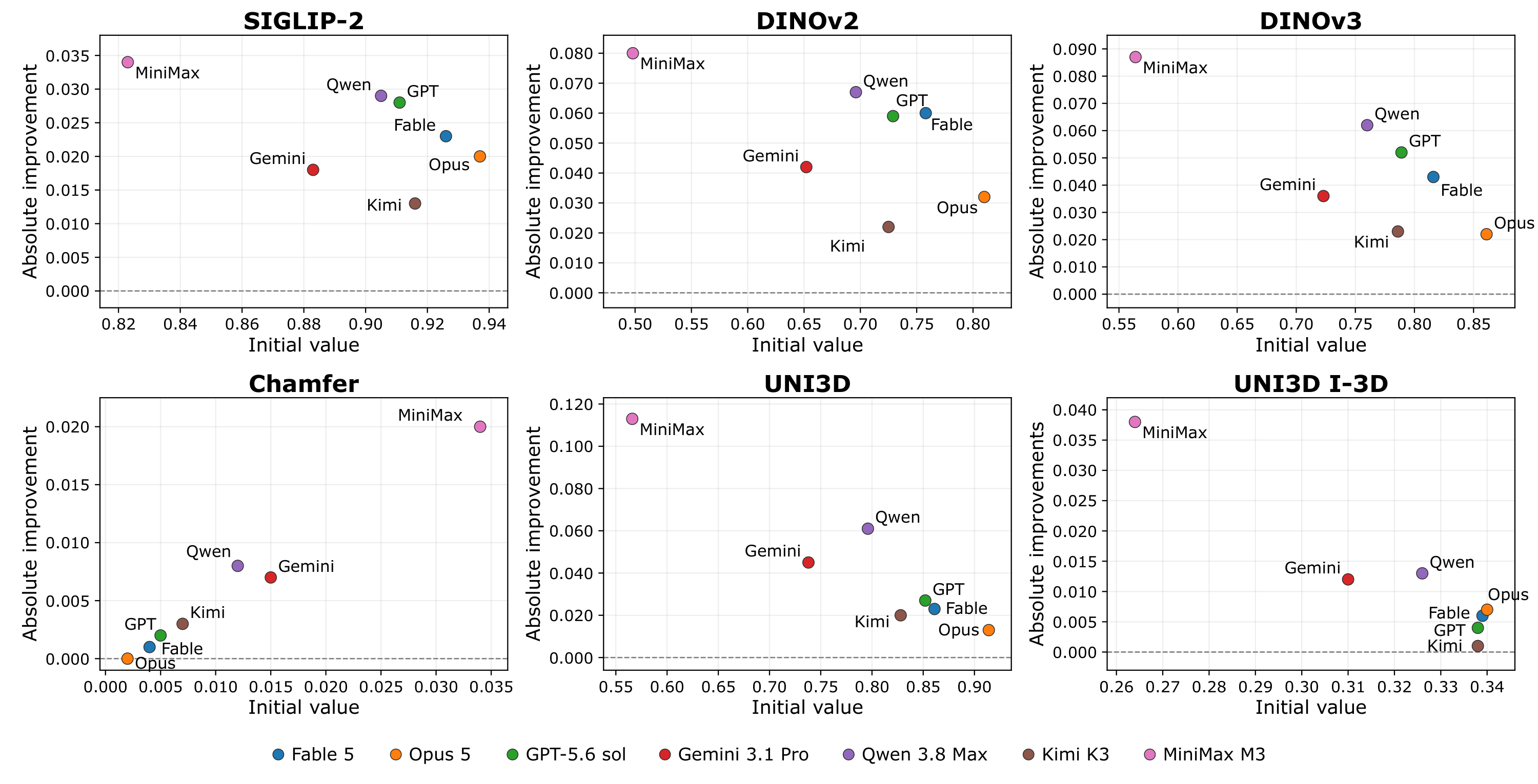
Initial versus final Uni3D improvement for agents in 3DHarnessBench
Prior baseline: initial quality and repair gains
Future work tests transfer to new operations.
First-project synthesis of the Télécom Paris research proposal46
Future programmeProposed evaluation

The programme should survive difficult tests

HypothesisTestEvidence against it
Explicit structure improves controlHeld-out edits with geometric constraintsNo gain over simpler representations
Verified interaction teaches reusable skillsUnseen task and program familiesImitation without transfer
Structure reduces system costCount all assets and client computationGains disappear under full accounting

A useful negative result should change the representation, supervision or scope.

Research proposal: risks, generalization and controlled comparisons47
Télécom Paris

Complementary expertise for the research programme

ConnectionResearch opportunityRelationship
Amal Dev Parakkat IMAGES teamExecutable 3D construction and evaluationExisting 3DHarnessBench collaboration
Kaouther MessaoudGeometry-grounded motion and video generationProposed collaboration
Stephan Alaniz · Jhony GiraldoFine-grained grounding and relational structureProposed collaboration
Enzo Tartaglione · Xiaoran JiangCompact models and Gaussian compressionProposed collaboration
Jean Le FeuvreGPAC streaming and end-to-end delivery costProposed collaboration
Kiwon Um · S2A group IDS DepartmentDifferentiable simulation and audio-driven animationProposed collaboration
Hi! PARISSeminars, summer school and internal callsChair attached to the post
Télécom Paris dossier, integration plan; proposed links distinguished from existing work48
Conclusion

Representations and feedback must support the task

Usable geometry exposes structure.
Semantic features identify what to change.
Execution and feedback test whether it worked.

The programme: From Video to Animatable and Efficient 3D Worlds.
The first project: verified trajectories for compact models that reconstruct and edit articulated objects.

The next step is to learn representations and operations together, with checks we can trust.

Bingchen Gong
bingchen.gong@lix.polytechnique.fr · gongbingchen@gmail.com

From Reconstruction to Reasoning: Structured 3D Representations49
FourieRFPublished

A 3D feature field built from lines and planes

Line feature vˣ(x) x × Plane feature Mʸᶻ(y,z) (y,z) = One 3D component at the query point (x,y,z)

T(x,y,z) = ∑r [vrx(x)Mryz(y,z) + vry(y)Mrxz(x,z) + vrz(z)Mrxy(x,y)]

T: feature grid · r: component index. Sum components in all three orientations.

Density and appearance come from compact factors. FourieRF controls the detail stored in each factor.

Gomez, Gong & Ovsjanikov · FourieRF · 3DV 2025B1
FourieRFPublished

FourieRF: bandwidth and optimization

bt = b₀ + tΔ,   Δ = (1 − b₀) / N

Conceptual linear schedule in the main method. N is its duration.

What changes

  • Filter every 1D and 2D tensor factor before field evaluation.
  • Use the prescribed mask at iteration t while differentiating the image loss.
  • Remove positional encodings from feature and view-direction decoder inputs.

What optimizes the field

  • Training-image supervision and total variation on density and appearance features.
  • Synthetic scenes: AdamW weight decay 0.2.
  • Real scenes: density-feature L1 penalty weighted 10⁻⁴, with zero weight decay.

The source has conflicting initial-bandwidth values and an inconsistent synthetic increment. Use the released implementation for exact reproduction.

Gomez, Gong & Ovsjanikov · FourieRF · 3DV 2025B2
FourieRFPublished

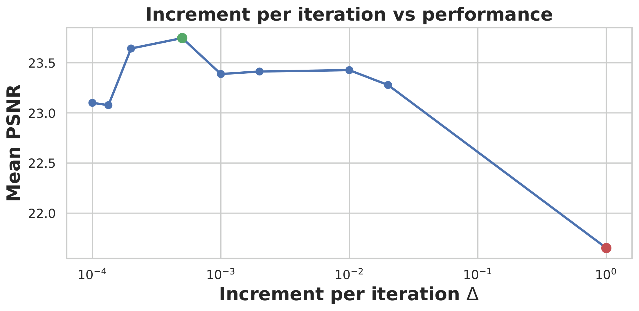
The rate of detail release matters

Blender, six input views. The frequency-increment axis is logarithmic.

Rapid release weakens regularization. Very slow release can underfit the fixed budget.

Gomez, Gong & Ovsjanikov · FourieRF · 3DV 2025B3
FourieRFPublished

FourieRF: protocol and scope

EvaluationInput viewsFourieRF PSNR
Blender: 8 scenes4 / 621.728 / 23.927 dB
LLFF: 8 scenes3 / 6 / 919.303 / 23.595 / 25.011 dB
  • Blender follows ZeroRF’s evaluation setup; LLFF follows RegNeRF’s.
  • 10,000 iterations; VM tensor factors in the main comparison.
  • No claim of recovering truly unobserved surfaces.
Gomez, Gong & Ovsjanikov · FourieRF · 3DV 2025B4
FourieRFPublished

FourieRF: interpreting the timing ratio

MethodRelative training time ↓4-view Blender PSNR ↑
TensoRF1.000
FourieRF-VM0.93021.728 dB
ZeroRF5.18121.940 dB
FreeNeRF35.710

5.57× training speedup over ZeroRF in this setup, with 0.212 dB lower PSNR.

10,000-iteration Blender timing comparison; TensoRF normalized to 1. RTX 4090.

Gomez, Gong & Ovsjanikov · FourieRF · 3DV 2025B5
FourieRFPublished

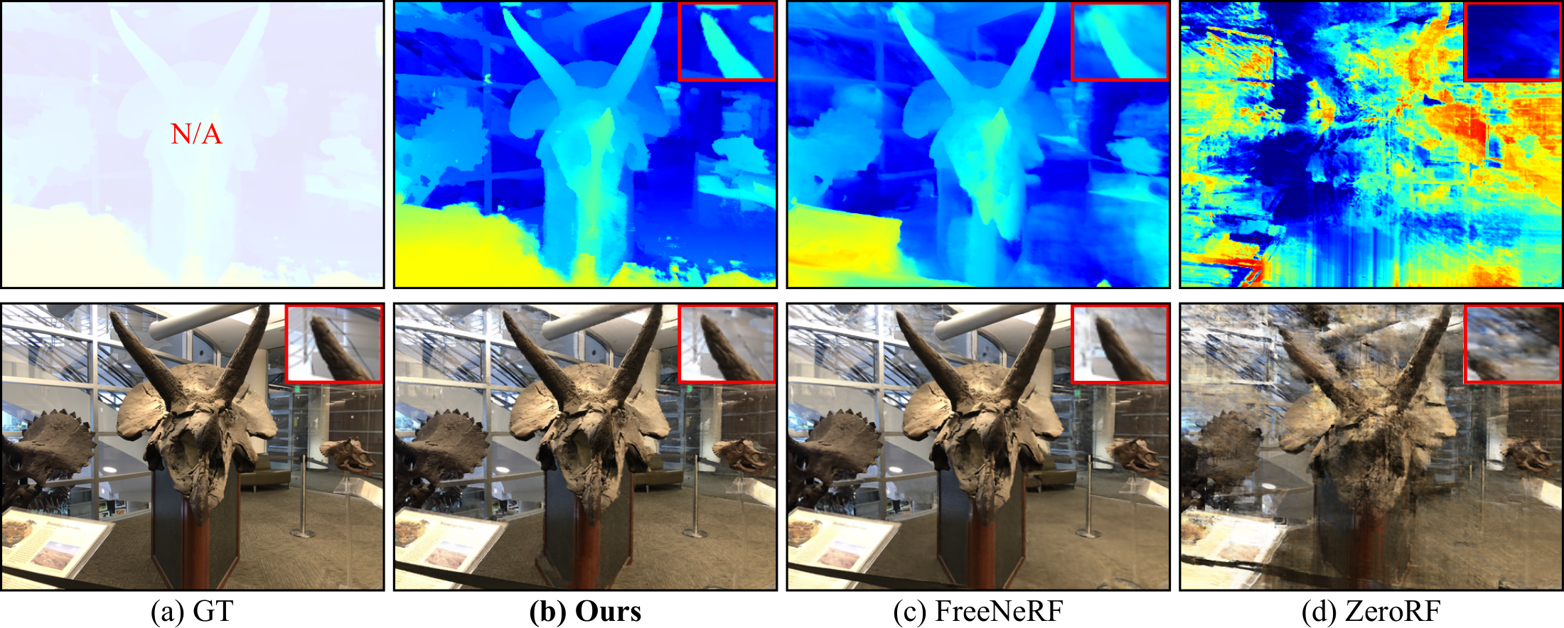
FourieRF: real-scene comparison

LLFF example: ground truth, FourieRF, FreeNeRF, ZeroRF. The reference has no ground-truth depth.

Competitive reconstruction does not imply the best PSNR or verified depth.

Gomez, Gong & Ovsjanikov · FourieRF · 3DV 2025B6
MILoPublished

MILo: losses and geometric evaluation

AblationTanks & Temples F1 ↑
Baseline0.41
+ Mesh depth0.46
+ Mesh normals0.44
+ Anti-erosion0.44
+ Interior regularization0.47
GOF integration0.49

Normal supervision improves selected surfaces visually even when rounded F1 decreases.

Guédon, Gomez, Maruani, Gong, Drettakis & Ovsjanikov · MILo · TOG 2025B7
MILoPublished

MILo: optimization and evaluation boundaries

IterationsTraining stage
0–3,000Photometric fitting and aggressive densification
3,000–8,000Normal regularization; Gaussian refinement
8,000–18,000Mesh supervision and selected pivots

Delaunay update: 500 iterations. Occupancy-label update: 200 iterations.

Mesh-rendering quality complements direct geometry metrics; it does not certify unseen surfaces.

Guédon, Gomez, Maruani, Gong, Drettakis & Ovsjanikov · MILo · TOG 2025B8
MILoPublished

MILo: preserving the surface and cleaning its interior

Preserve selected Gaussian centers

erosion = ∑g∈GDel max(0, fμg)

GDel: Gaussians selected for triangulation
fμg: signed value at a Gaussian center

Penalize positive center values. Keep a negative sample inside thin structures.

Suppress unsupported interior surfaces

interior = ∑p op H(σ(−fp), op)

op = 1 when pivot p lies behind all visible mesh depths
H: binary cross-entropy · σ: sigmoid

Supervise only interior-labeled pivots. Refresh labels every 200 iterations.

ℒ = ℒvol + λMDMD + λMNMN + λerosionerosion + λinteriorinterior

λMD = λMN = 0.05 · λerosion = λinterior = 0.005 in the reported implementation.

Guédon, Gomez, Maruani, Gong, Drettakis & Ovsjanikov · MILo · TOG 2025B9
MILoPublished

A zero crossing gives a differentiable surface vertex

pₐ, fₐ < 0 v, f = 0 pᵦ, fᵦ > 0 Inside pivot Surface vertex Outside pivot

v = (fₐpᵦ − fᵦpₐ) / (fₐ − fᵦ)

Moving either pivot or changing its signed value moves the extracted surface.

Mesh lossesSurface vertices v
Signed values f
Gaussian geometry μ, R, s

Arrows show the gradient path. Discrete Delaunay connectivity updates every 500 iterations.

Guédon, Gomez, Maruani, Gong, Drettakis & Ovsjanikov · MILo · TOG 2025B10
MILoPublished

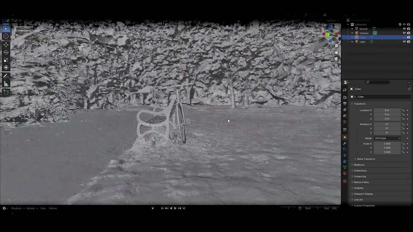
Inspecting recovered thin structures

Original supplementary video: exported bicycle and bench mesh in Blender.

Changing the viewpoint exposes details that a single attractive rendering can conceal.

Guédon, Gomez, Maruani, Gong, Drettakis & Ovsjanikov · MILo · TOG 2025B11
From Blobs to SpokesPublished

Spokes: oriented fields and surface extraction

Original paper diagram: oriented Gaussians supply normal and vacancy fields, with pivot-based Marching Tetrahedra and optional Primal Adaptive Meshing

Two pivots per Gaussian
Use the center and an outward-displaced point for tetrahedral surface extraction.

Primal Adaptive Meshing (PAM)
Resample and project vertices to control mesh resolution independently of Gaussian count.

Tanks & Temples · mean F1 ↑ · six scenes

MethodUniform samplingVirtual scan
MILo0.340.42
Spokes (2 pivots)0.480.53

Both methods evaluated with the Spokes paper’s protocols.

Vacancy and normal fields are estimated in practice. The table reports the two-pivot variant; PAM is optional.

Gomez*, Guédon*, Maruani, Gong & Ovsjanikov · From Blobs to Spokes · ECCV 2026 · Fig. 3 and Table 1B12
MILoPublished

MILo: fewer vertices and smaller meshes

MethodMesh vertices ↓Mesh size ↓Training time ↓
GOF16.49 M600.0 MB93 min
RaDe-GS14.75 M592.0 MB42 min
MILo base4.36 M179.6 MB50 min
MILo dense6.89 M276.1 MB110 min

Tanks & Temples resource table; RTX 4090. Base/dense use the RaDe-GS backbone. Legacy vertex-based F1: MILo 0.47 (base) and 0.49 (dense); GOF 0.46, RaDe-GS 0.40.

Mesh size and geometric accuracy are separate claims. Compare accuracy with a common surface-sampling protocol.

Guédon, Gomez, Maruani, Gong, Drettakis & Ovsjanikov · MILo · TOG 2025B13
ZeroKeyPublished

ZeroKey: localization thresholds and comparison scope

Method0.010.050.10
B2-3D · few-shot, 62 views20.2957.7270.57
B2-3D · few-shot, 26 views14.3944.1156.90
GPT-4o localizer0.486.0420.73
CLIP-DINOiser1.419.8025.56
StablePoints5.8019.9138.22
Binary back-projection5.8429.8154.64
ZeroKey · 26 views13.1656.6079.43

KeypointNet: airplane, chair and table. IoU (%) at geodesic thresholds.
StablePoints receives the ground-truth keypoint count; benchmark text descriptions are manually assigned.

Gong et al. · ZeroKey · ICCV 2025 supplement · Table 3B14
ZeroKeyPublished

ZeroKey: distinguish dense agreement from isolated votes

Ordinary distance treats an isolated pair like a well-supported cluster.

dm(a,b) = max{corek(a), corek(b), ‖a − b‖}

corek(a)
Distance from candidate a to its kth nearest neighbor.

Isolated candidates have large core distances, even if two happen to be close.

HDBSCAN on pooled 3D candidates

  • Use the Gaussian soft-voting weights.
  • Find stable dense clusters across views.
  • Fix minPts k = 10 in the experiments.

Spatial density separates repeated semantic instances from inconsistent predictions.

Gong et al., ZeroKey, ICCV 2025B15
ZeroKeyPublished

A named point is a localization problem

“Point to the corners of the chair back.”

  • Input: a known mesh and a text query
  • Output: named locations on its surface
  • No task-specific 3D keypoint training

Semantic recognition still needs precise spatial grounding.
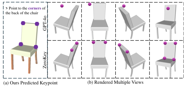
The same chair query in multiple rendered views
Gong et al., ZeroKey, ICCV 2025B16
ZeroKeyPublished

Use known depth to lift an uncertain image point

Image-language predictions for the same chair-corner query
A small image error can cross a silhouette or a depth discontinuity.

Cache the mesh depth while rendering.
Each valid pixel maps to a visible 3D surface point.

xj(u) = RjT[Dj(u) Kj−1ũ − tj]

u: pixel; ũ: homogeneous pixel
D: camera-depth map; K, R, t: camera parameters

Lift an h × h neighborhood, reject background pixels, then average its valid 3D points.

Gong et al., ZeroKey, ICCV 2025 · method: depth-cached back-projectionB17
ZeroKeyPublished

Sparse semantic handles leave gaps

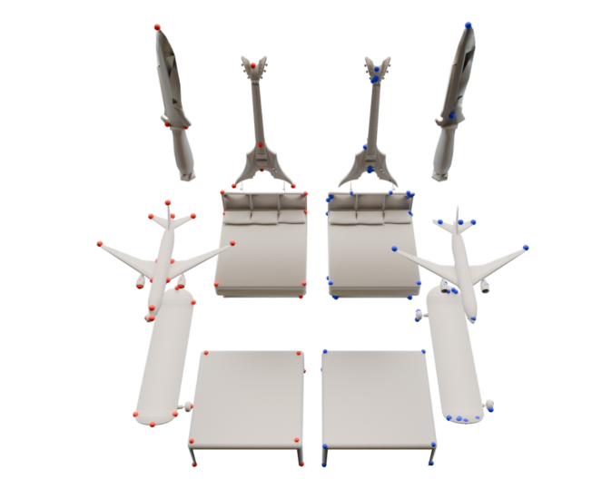
Selected named keypoints across different shapes

What represents the surface between the points?

  • Repeated model calls make dense querying costly.
  • Ambiguity and symmetry remain.
  • Editing and segmentation need local features across the shape.

The next step is to learn language-aligned features directly in 3D.

Gong et al., ZeroKey, ICCV 2025B18
PatchAlign3DPublished

PatchAlign3D: where the two training signals come from

Pseudo-part annotations

  • 32,052 Objaverse shapes: 28,827 train / 3,225 validation.
  • 10 views per shape → SAM masks → Gemini 1.5 part names.
  • Back-project to 3D; retain overlapping labels.
  • Over 2 million annotations, 761 categories.

Training and representation

  • Stage 1: frozen DINOv2 visual targets.
  • Stage 2: OpenCLIP ViT-bigG-14 text embeddings.
  • 100 epochs per stage; batch size 32.
  • Learn τ and b, initialized at 0.1 and −10.

Random rotations, translations, scaling and point jitter support generalization.

Hadgi et al., PatchAlign3D, CVPR 2026B19
PatchAlign3DPublished

PatchAlign3D: build a stable visual target before training

Rendered feature mapsBicubic upsampling to image resolution
Visible surface pointsAverage observations across views
Cached patch targetsAverage features within each patch

d(x) = 1/|V(x)| ∑r ∈ V(x) Frr(x))

di = 1/k ∑x ∈ Pi d(x)

V(x): views observing x; Fr: DINOv2 feature map; πr: camera projection; k: points per patch.

L2D = 1/G ∑i [1 − cos(h2D(zi), di)]

zi: patch token; h2D: visual projection; G: number of patches.

Match each online patch center to the nearest cached center before applying the cosine loss.

Hadgi et al., PatchAlign3D, CVPR 2026 · visual-target constructionB20
PatchAlign3DPublished

PatchAlign3D: benchmark scope and exceptions

BenchmarkPatchAlign3D mIoUComparator mIoUQualification
ShapeNetPart56.9COPS 25.6Laptop: 61.1 vs COPS 63.3
FAUST67.8Find3D 63.2Torso: 49.7 vs Find3D 52.0
PartNetE41.4COPS 27.0PartSLIP reports 36.4 cIoU
ScanObjectNN22.7Find3D 18.8Noise and clutter remain difficult
Objaverse unseen35.61Find3D 34.6Author-defined 14-category split

Different datasets and metric definitions support different conclusions.

Hadgi et al., PatchAlign3D, CVPR 2026B21
PatchAlign3DPublished

PatchAlign3D: selected segmentation examples
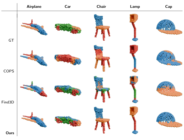
Original ShapeNetPart examples with all displayed baselines

Spatial coherence
Many predicted regions follow recognizable parts.

Boundary limitations
The car remains a useful counterexample.

Qualitative examples illustrate behavior. Aggregate tables determine the measured gain.

Hadgi et al., PatchAlign3D, CVPR 2026B22
PatchAlign3DPublished

Stronger part segmentation at feed-forward speed

ShapeNetPart, point-cloud methods. Reported IoU (%) and inference time.

MethodmIoUcIoUSeconds / shape
COPS25.632.21.38
Find3D23.323.90.4
PatchAlign3D56.953.10.4

+31.3 percentage points mIoU over COPS. The reported runtime matches Find3D.

mIoU averages instances. cIoU averages categories. Timings refer to the paper’s evaluation.

Hadgi et al., PatchAlign3D, CVPR 2026B23
PatchAlign3DPublished

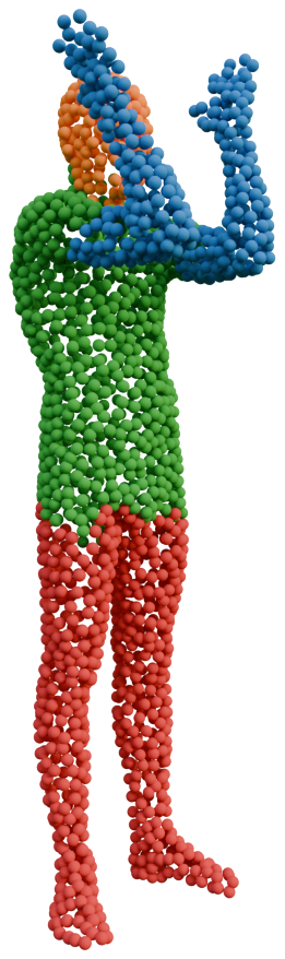
Transfer improves, but domain shift remains
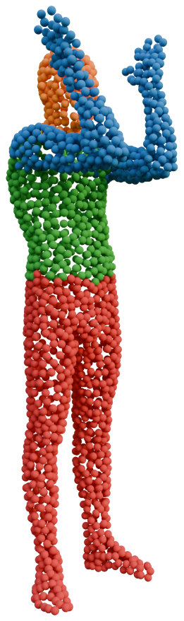
FAUST ground truth

Ground truth

PatchAlign3D prediction

PatchAlign3D

A FAUST pose, with visible boundary errors
FAUSTmIoU (%)
COPS30.4
Find3D63.2
PatchAlign3D67.8

Real scanned objects are harder.
ScanObjectNN: 22.7 mIoU versus Find3D’s 18.8.

Improvement does not remove the robustness gap.

Hadgi et al., PatchAlign3D, CVPR 2026B24
PatchAlign3DPublished

PatchAlign3D: patch encoding and point-level inference
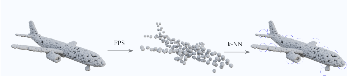
Point cloud to farthest-point centers and overlapping local neighborhoods
2,048 XYZ points → 128 FPS centers → 32 nearest neighbors per patch
Local encodingPointNet(Pi) + MLP(ci)Pi: patch points; ci: center
Context across patches12 transformer layers128 output patch tokens
Text projectionCompare each patch with part namesOpenCLIP ViT-bigG-14 text embeddings

ŷ(x) = arg maxj ⟨zi(x), tj⟩,   i(x) = arg mini ‖x − ci

z: text-aligned patch feature; t: part-name embedding. Each point inherits its nearest center’s label.

Hadgi et al., PatchAlign3D, CVPR 2026B25
Appendix · feedback learningOngoing work

What is trained, and what counts as supervision?

VLM-reward setting

  • Source points are provided.
  • DINOv3 is pretrained and frozen apart from LoRA.
  • The VLM scores sampled target matches.
  • Target annotations are used for evaluation, not the reward.

Separate diagnostic settings

  • Ground-truth PCK reward is supervised.
  • Geometry-aware fusion changes the feature stack.
  • Cat-only and all-category training are different regimes.
  • Peak validation is not held-out test performance.
Is It a Good Match? · experimental settingsB26
Appendix · feedback learningOngoing work

Training details: stochastic updates and residual feature fusion

Policy update

t = −(1/B)(rt − bt) log πθ(qt)

  • Temperature τ = 0.1; EMA rate 0.01.
  • Accumulate B = 10 samples per Adam step.
  • Clip gradient norm at 1.0.
  • Skip invalid scores; retain valid zero scores.

Optional geometry-aware features

Cached SD v1.5 features: 640 + 1280 + 1280 channels.
Live DINO ViT-B features: 768 channels.

F̂ = φ(FDINO) + a · AggNet([FSD; FDINO])

φ: DINO projection; a: learnable fusion gate.
Fuse at a shared 60 × 60 feature grid.
Train LoRA and the aggregation network.
The residual branch preserves the DINO signal.

Gong et al. · method and implementation appendixB27
Appendix · feedback learningOngoing work

Transfer is measurable, but not uniform

Test categoryFrozen DINOv3Geo-aware, 3 seedsΔ PCK
Cat, trained category73.2777.74 ± 0.64+4.47
Bird80.4583.04 ± 0.27+2.59
Cow72.0673.31 ± 0.45+1.25
Sheep61.5062.64 ± 0.42+1.14
Dog61.8962.82 ± 0.09+0.93
Horse65.0364.32 ± 0.17−0.71
Person65.6264.50 ± 0.56−1.12

SPair-71k test · cat-trained only · bbox PCK@0.10. Other-category mean gain: +0.68; plain LoRA: +0.02.

Is It a Good Match? · cross-category test tableB28
Learning from feedbackOngoing work

Alternative updates under the same judge budget

MethodPCK ↑
Frozen DINOv376.19
Top-K + LoRA78.06 ± 0.04
DPO + LoRA79.09
REINFORCE + LoRA78.94 ± 0.14

SPair-71k cat validation · bbox PCK@0.10
Kimi reward · 3 seeds where uncertainty is shown.

+2.75 points
over the frozen backbone

The gain demonstrates useful feedback in this regime.

REINFORCE exceeds the listed Top-K setting; it does not establish superiority to DPO.

Gong et al. · current manuscript, Table 1 · cat-only validationB29
Learning from feedbackOngoing work

Semantic feedback still needs a geometry-aware representation
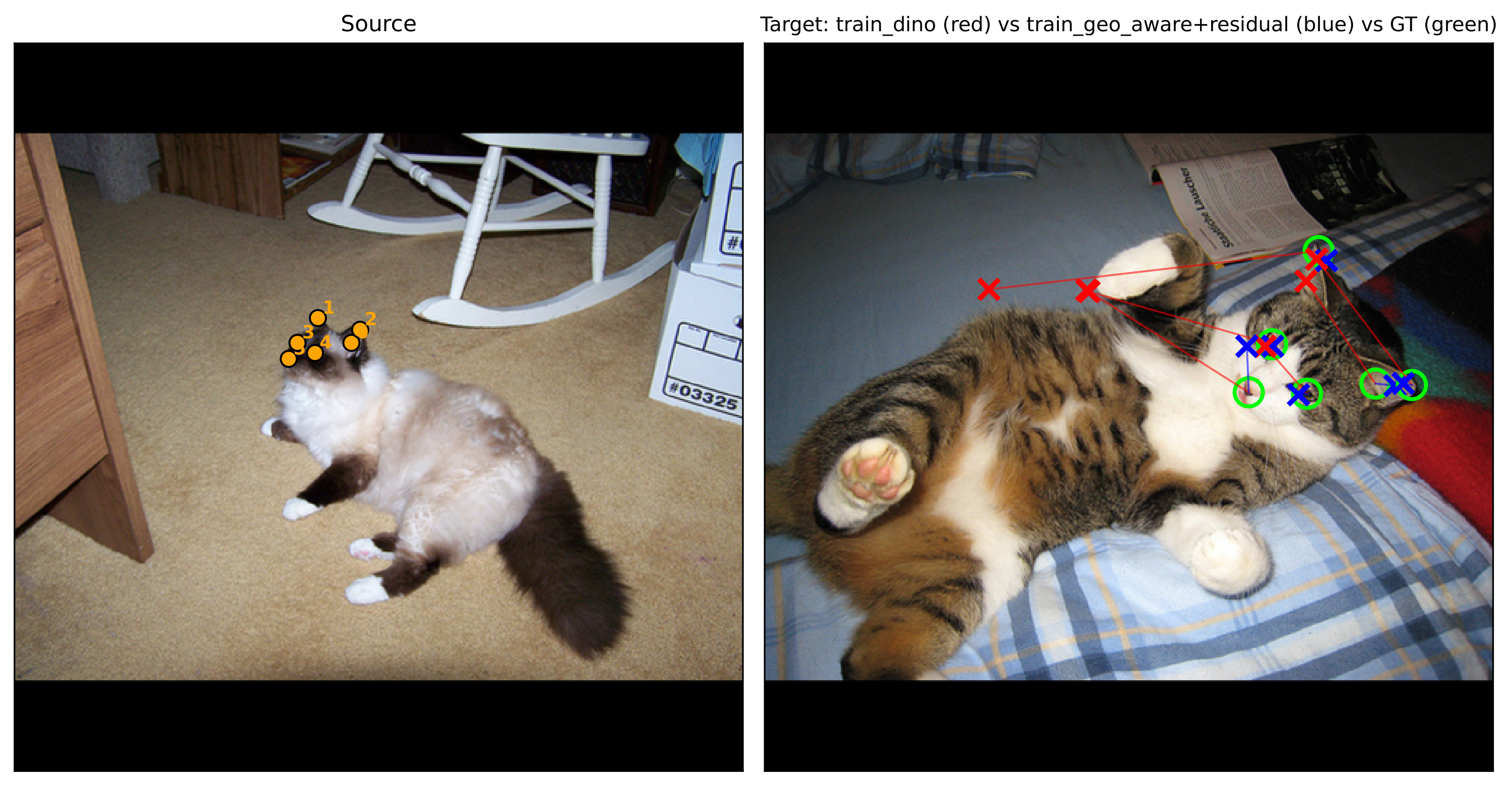
Cat correspondence example comparing plain DINO matches in red, geometry-aware matches in blue and ground truth in green
One SPair cat test pair · red: plain DINO pipeline · blue: geometry-aware variant · green: ground truth

Adding geometry-sensitive features can help resolve symmetry. This is an architectural comparison, not an isolated reward ablation.

Gong et al. · manuscript appendix, symmetry exampleB30
Learning from feedbackOngoing work

Visual inference after reward training

Training

Visual proposal → VLM feedback
→ adapted visual features

Semantic supervision is expensive
but can be amortized.

Inference

Two images + source point
→ feature matching → target point

No VLM call.
26.3 FPS reported for the plain pipeline.

Reported timing: 512² input, RTX A6000. Geometry-aware timing uses cached SD features and is a different pipeline.

The trained adapter keeps inference visual; the VLM cost is paid during learning.

Gong et al. · inference timing and deployment designB31
Appendix · executable reconstructionPreliminary update

Uni3D similarity across all reported agents and settings

AgentSingle viewFour viewsActive visualFull 3D
Fable 5.733.764.832.884
Opus 5.725.748.871.927
GPT-5.6 Sol.715.745.823.879
GPT-6 Astra*.794.842.912.956
Kimi K3.678.713.819.848
Qwen 3.8 Max.740.768.809.857
Gemini 3.1 Pro.728.753.691.783
MiniMax M3.495.577.482.679

↑ Higher similarity. * Preliminary unpublished aggregate update; Astra run coverage and complete protocol parity remain unverified.

3DHarnessBench · main_result-update.tex · UNI3D columnB32
Appendix · executable reconstructionOngoing work

The harness changes the observation and interaction protocol

SettingTarget accessTarget geometryRefinement
Single view1 fixed imageHidden3 rounds
Multi-view4 fixed imagesHidden3 rounds
Active VisualCamera / viewport toolsBlocked by allowlistAgent-directed
Full 3DUnconstrained Blender toolsAvailable to queryAgent-directed

100 sampled objects from 3DCodeBench.
Original procedural programs are withheld.

Active Visual separates target and reconstruction processes.
Full 3D prohibits copying the target.

3DHarnessBench · protocol table and benchmark formulationB33
Appendix · executable reconstructionOngoing work

Evaluation conventions determine what a score can mean

Geometric alignment

Sample 8,192 surface points per mesh.
Center each cloud and scale to the unit sphere.

CD = minR ∈ R₂₄ dsym(RX, Y)

dsym: mean squared nearest-neighbor distances in both directions.
R₂₄: the 24 right-handed axis-aligned rotations.

Translation, scale and these rotations are discounted.

Complementary checks

Appearance: four 512² renders; match views by the best one-to-one assignment.

etopo = Σi=0..2iGT − βirec| / Σi=0..2 βiGT

Topology: median across objects.
Other quality metrics: mean across objects.

No loadable mesh: zero similarity; Chamfer penalty of 1.5 × the worst valid value in that run.

3DHarnessBench · supplementary experimental settings / metricsB34
Appendix · executable reconstructionOngoing work

Ablations separate observation quality from evidence quantity

Agent / evidence settingChamfer ↓Uni3D ↑
Gemini · four fixed views.0165.7609
Gemini · Active Visual.0234.6776
Gemini · normalized viewport.0186.7321
Gemini · Fable inspection views.0191.7605
MiniMax · Active Visual.0798.3722
MiniMax · normalized viewport.0240.6148

Ten-target ablation: better observations recover much of the lost performance, with metric-dependent outcomes.

3DHarnessBench · observation-interface ablation · 10 targetsB35
Executable 3D hypothesesOngoing work

The agent chooses both an observation and a program update

at ∼ πθ(· | Ht)   Ht: instructions, observations and previous actions

Acquire evidenceNew view or geometric queryot: image; plus measurements in Full 3D
Revise the hypothesisBlender program PtParts, dimensions, transforms and materials
Execute and inspectĜt = E(Pt)E: Blender execution; compare with the target

Active Visual

Separate target and reconstruction processes.
Target tools allow camera and viewport control.
Direct geometry access is blocked.

Full 3D Interaction

Query dimensions, transforms and distances.
The agent decides what to measure and when.
Copying the target is prohibited by instruction.

Evaluate the final executed object ĜT, plus the interaction needed to obtain it.

Liu et al. · benchmark formulation and target-access protocolsB36
Executable 3D hypothesesPreliminary update

More access helps only when an agent can use it

0.00.20.40.60.81.0Uni3D similarity ↑GPT-6 Astra*Opus 5Gemini 3.1 ProSingle viewFour fixed viewsActive visualFull 3D* Astra: preliminary, unpublished aggregates; matched coverage and protocol not yet verified.
Selected agents · original seven-agent results plus preliminary Astra aggregates.

Active inspection can improve or degrade reconstruction. Full 3D access includes explicit geometric evidence.

3DHarnessBench · main_result-update.tex · Astra preliminaryB37
Executable 3D hypothesesOngoing work

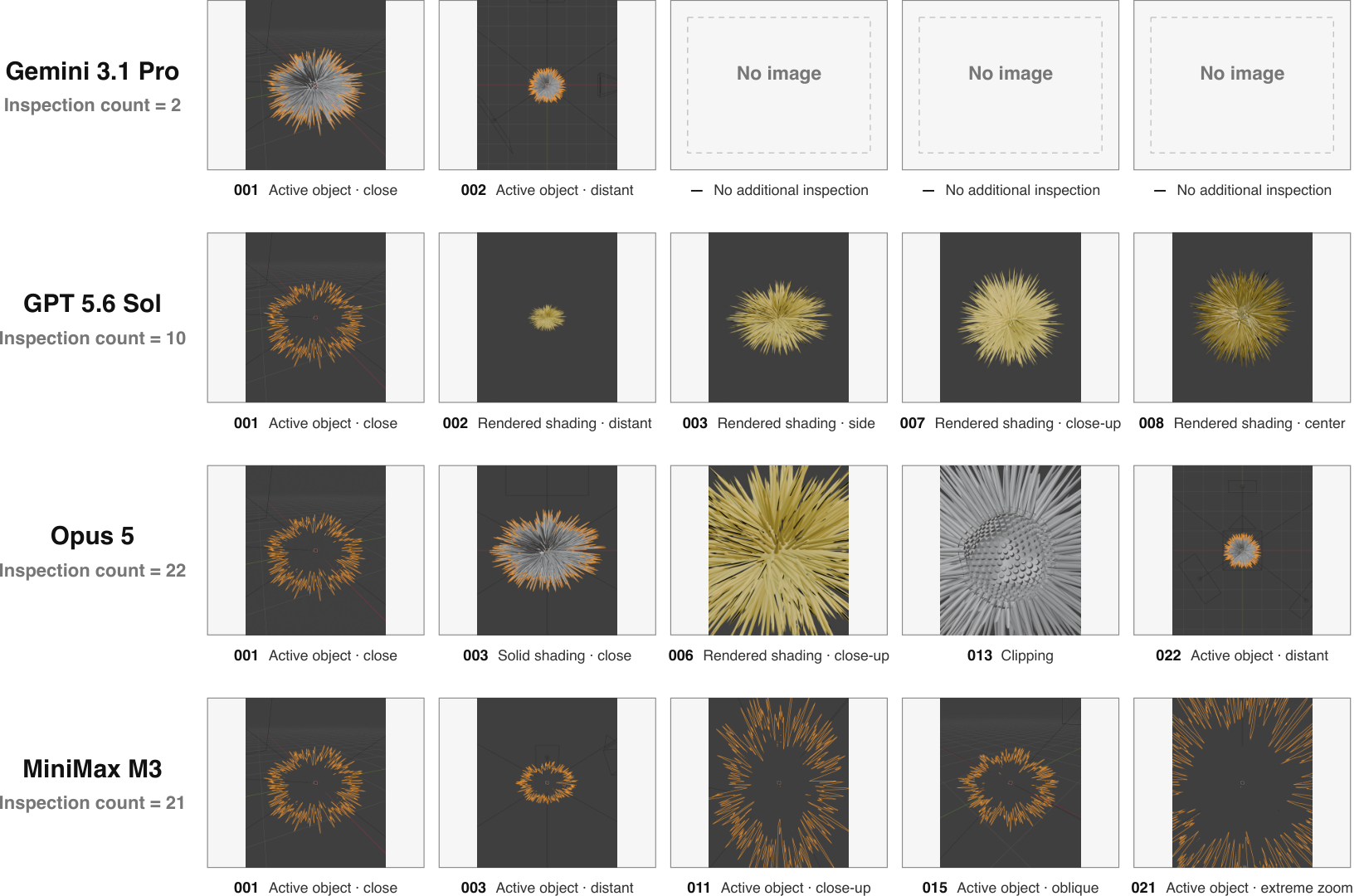
Observation quality affects reconstruction

Gemini inspection sequence with two observations
Two Gemini inspections on this target.
Selected views from 22 Opus inspections of the same target
Selected views from 22 Opus inspections of the same target.

On 10 ablation targets, viewport normalization raises MiniMax Uni3D: 0.3722 → 0.6148.

3DHarnessBench · inspection examples and 10-instance ablationB38
Executable 3D hypothesesOngoing work

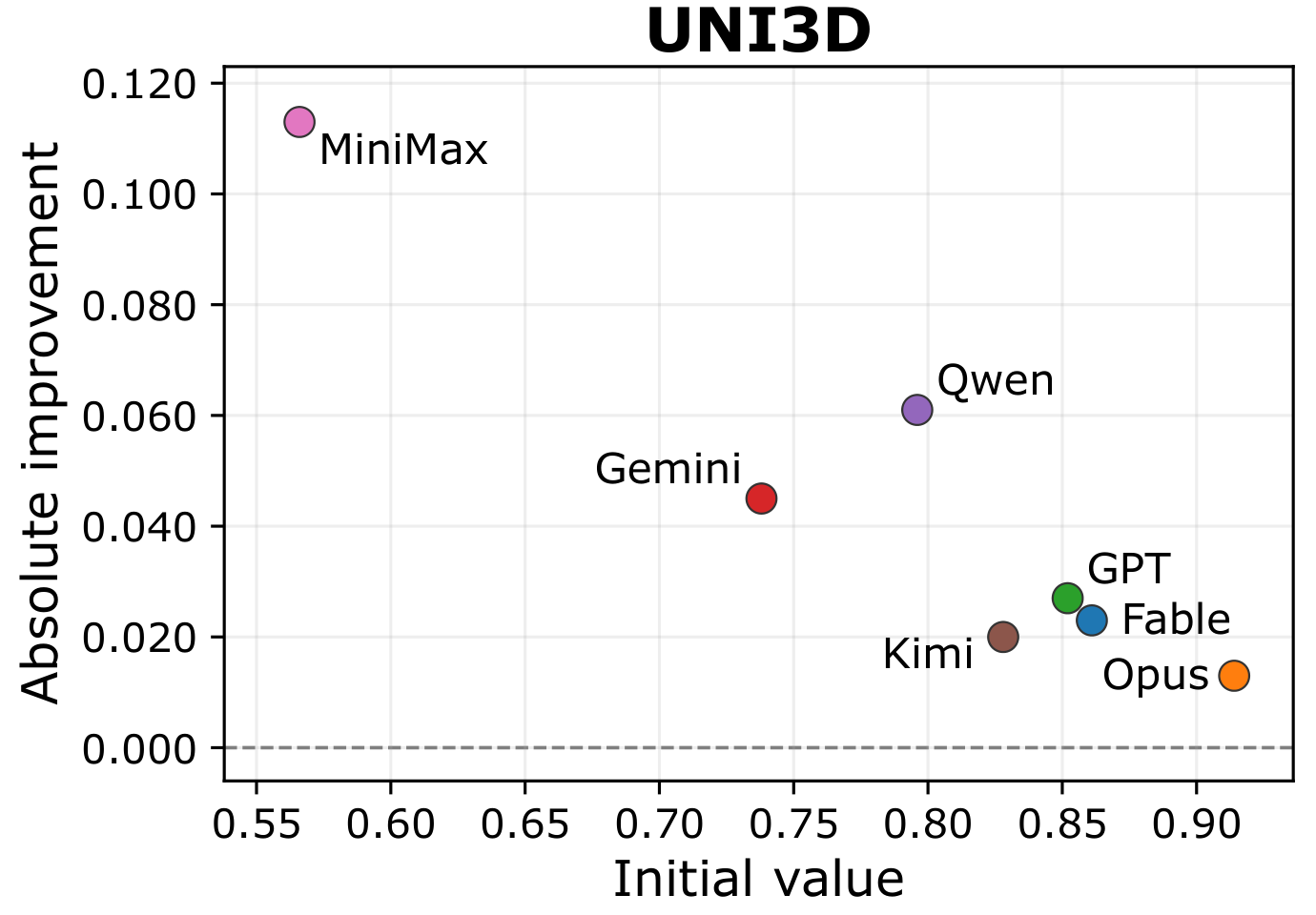
A strong first reconstruction and a strong repair policy differ

Scatter of initial Uni3D score versus absolute improvement from refinement for seven agents
Original seven-agent study · Full 3D interaction · no Astra repair data.

Measure both abilities

  • Opus starts high and gains modestly.
  • MiniMax improves substantially from a weak start.
  • Qwen combines a stronger start with larger repair gains.

A larger gain does not imply a better final model.

3DHarnessBench · initial-finalv2 · original seven-agent studyB39
Appendix: contributions

Research ownership and collaboration

ProjectDocumented contribution
FourieRF / MILo / SpokesCoauthorship, mentoring of Diego Gomez, MILo code contributions and LIX/GRAPHDECO collaboration
ZeroKeyConceived, implemented and evaluated the first-author project
PatchAlign3DJoint research with Souhail Hadgi and collaborators
Is It a Good Match?Scientific lead since April 2026, experiments and manuscript
3DHarnessBenchExperiment guidance, project coordination, TaskSolver and restricted Blender interface
Publication list and activity report, September 2026B40
Appendix: teaching

Teaching and mentoring

Experience

  • Teaching assistant for eight HKU courses
  • Certificate in Teaching and Learning in Higher Education
  • Forthcoming MVA geometry teaching appointment
  • Research mentoring across vision and graphics

Contribution at Télécom Paris

  • Graphics, geometric learning and neural 3D representations
  • Projects linking implementation to measurable evidence
  • Teaching in English, with a commitment to French within two years
Télécom Paris teaching statement and activity report, September 2026B41
Appendix: research developmentProposed work

A staged research programme

StageScientific focusDevelopment
First yearControlled static/articulated tasks, verified trajectories, compact baselinesInitial student project and reproducible releases
Second yearTransfer to new operations and richer dynamicsCollaborative funding and industrial research links
Third yearIntegrated reconstruction, animation and delivery evaluationBroader partnerships and HDR preparation

Resources and extensions follow demonstrated progress on the core tasks.

Télécom Paris research proposal, team building and timelineB42